Historical Aspects¶

The quantum Hall effect is a remarkable phenomenon discovered experimentally in which the Hall conductivity of a two dimensional system of electrons is found to have plateaus as a function of variables which determine the number of electrons participating in the effect.

The integer quantization of the Hall conductance was originally predicted by Ando, Matsumoto, and Uemura in 1975, on the basis of an approximate calculation which they themselves did not believe to be true![7]

Several researchers subsequently observed the effect in experiments carried out on the inversion layer of MOSFETs. It was only in 1980 that Klaus von Klitzing, working at the high magnetic field laboratory in Grenoble with silicon-based samples developed by Michael Pepper and Gerhard Dorda, made the unexpected discovery that the Hall conductivity was exactly quantized. For this finding, von Klitzing was awarded the 1985 Nobel Prize in Physics.

What alerted von Klitzing to the effect was the insensitivity to the fine-tuning of the magnetic field strength. He “switched on” the field to apply it to a device through which a fixed current was flowing stabilized by a constant current source, and observed that when things stabilized, a digital voltmeter always showed the same Hall voltage across the sample to many significant figures. (The story is told that he first thought the voltmeter was broken!) Of course, each time the magnetic field was “turned on” was different, so the final field would never have been the same on each run of the experiment, and certainly would never have “accidentally” taken the precise “magic value” of the naive explanation. It is fortunate that von Klitzing switched on the magnetic field with a fixed current through the sample, rather than switched on the current at fixed field, as the coincidence of the unchanged digital voltmeter readings would then never have happened. [4]

Theoretical aspects [8,6]¶

The Classical Hall Effect¶

The original, classical Hall effect was discovered in 1879 by Edwin Hall. It is a simple consequence of the motion of charged particles in a magnetic field.

The setup for the same is as follows, consider a rectangular bar with thickness, t, Length L, and width W, as shown in Fig 1. Now a constant current along the \(x\) axis is passed. When a magnetic field is applied along the \(z\) axis (\(B_{z}\)), the charges in the current experience a force (the Lorentz force).

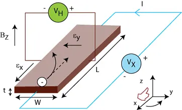
In the absence \(B_{z}\), the charges follow approximately straight paths. However, when \(B_{z}\) is applied, their paths get curved, in this way moving charges aggregate on one face of the material. This leaves equal and opposite charges exposed on the other face, where there is a scarcity of mobile charges. The separation of charge establishes an electric field that opposes the migration of further charge, so a steady electric potential is established for as long as the charge is flowing. This is called the Hall voltage \(V_{H}\).

The Hall voltage \(V_{H}\) can be derived by using the Lorentz force given that, in the steady-state condition, charges are not moving in the y-axis direction. \(\vec{{F}}=q(\vec{E}+\vec{vx\vec{B_{z}}})\) , Now \(\vec{F}=0\implies0=E_{y}-v_{x}B_{z}\) also \(E_y=-\frac{V_H}{w}\) thus on substituting these values we get :

This shows that \(V_{H}\) is proportional to \(B_{z}\), this result is used in commercial hall sensors which are used to measure magnetic field.

However one must note that the result drawn are for the the simple case with no impurities. Otherwise we will have to include the scattering effects. on doing so the previus equation gets modified as

where \(\tau\) is called the scattering time. Thus \(R_{H}\) called the Hall resistance is defined as

where n is the carrier constant.

Thus the measurement of Hall Coefficient gives the following information about the material

1. Carrier concentration , n

2. The sign determines the carriers are holes or electrons.

Experimental verification of hall effect.[5]¶

An experiment was performed to measure the charge density of Germanium used as Hall Probe. The experiment was performed under the guidance of Sharvari Kulkarni P.

The current passing through sample I, was kept constant at 10mA. The Hall Voltages \(V_{H}\) were measured for different values of Magnetic field. For each value of magnetic field, four readings corresponding to different geometric orientations were considered. This is essential due to presence of other thermal and galvanometric transport effects . The data and graphs are as following:

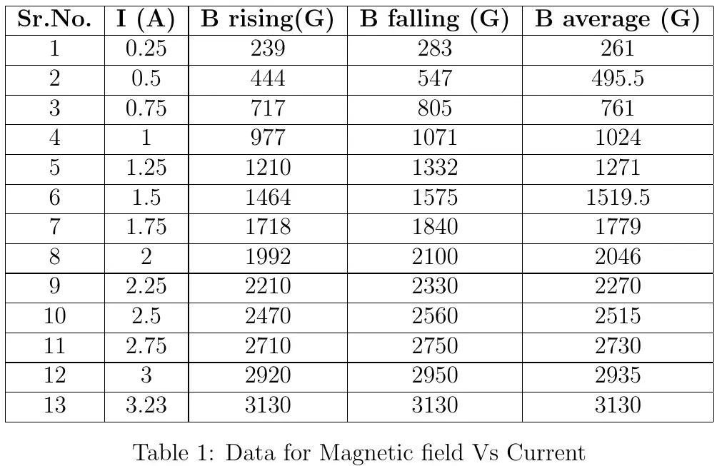
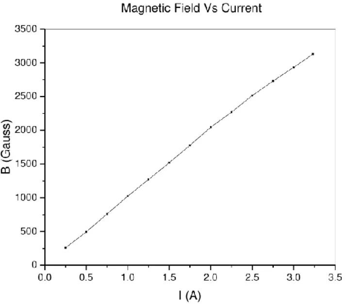
Part-1: The value of magnetic field corresponding to particular current was determined and plotted. Two readings corresponding to single current value specifies the values during increment and decrement of current viz. to minimize the error.

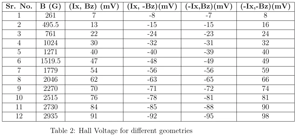
Part-2: The values of Hall Voltages are measured for different geometrical combinations.The data obtained is as follows -

Corresponding graphs are plotted here.

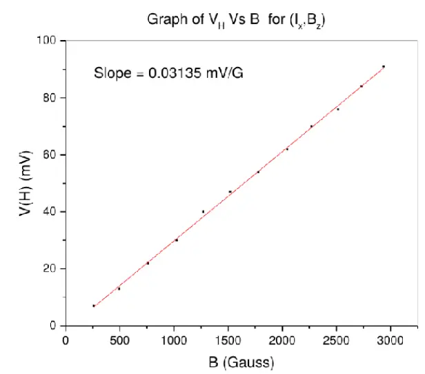
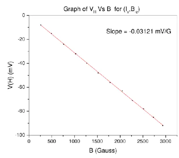
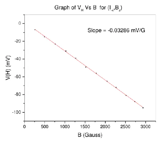
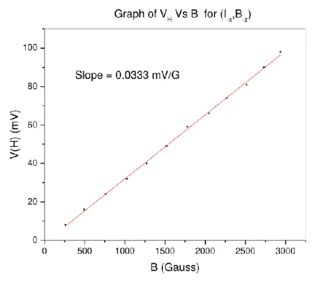
From all these graphs, the average value of slope is 0.03218 \(\frac{mV}{Gauss}\) . We have sample current equal to 10mA and sample length as 5mm.

1. Hence the value of Hall Coefficient is 0.1609 \(\frac{m^{3}}{C}\).

2. Positive sign implies that majority carriers are holes.

3. From this value, the carrier concentration can be calculated as \(n=3.879x10^{19}m^{-3}\)

Quantum Hall Effects¶

In the previous section we saw details about the Hall effect mainly that Hall Voltage is proportional to the magnetic field.

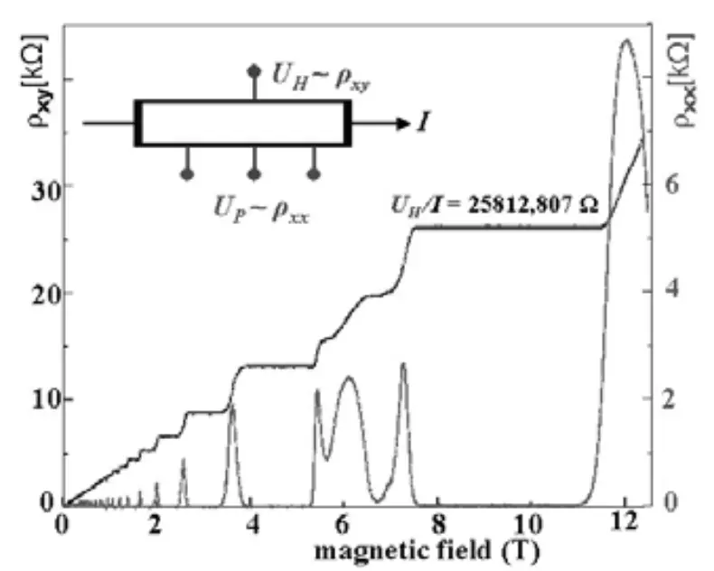
Hall effect is easily observed in room temperature and relatively low magnetic field. If the same setup is now taken down to low temperatures (typically around 1-5 K) and high magnetic field (greater than few Tesla) we see a non linear relation between Hall conductance and Magnetic field. We see some sort of quantization of Hall conductance. The observed resistivity is shown in next figure.

[8]

On observing the graph and a little bit of theoretical calculations one can deduce the following:

• Both the Hall resistivity \(\rho_{xy}\) and the longitudinal resistivity \(\rho_{xx}\) exhibit non linear behavior.

For lower magnetic field Transverse resistance varies linearly but after certain limit it changes step-like with integer multiples of \(\frac{\hbar}{e^{2}}\) with some plateau region in between.

• On these plateau, the resistivity takes the value

The value of \(\nu\) is measured to be an integer to an extraordinary accuracy —- something like one part in \(10^{9}\) .

The quantity\(\frac{\hbar}{e^{2}}\) is called the quantum of resistivity (with value 25.8128075 k )

• The longitudinal resistance has zero value otherwise except at a point where \(\rho_{xy}\) jumps from one plateau to another.

• The center of each plateau occurs at a point when magnetic field takes a value

  $$B=\frac{hn}{\gamma e}=\left(\frac{n}{\gamma}\right)\phi_{0}$$

Where, n is density of states of electrons and \(\phi_{0}=\frac{\hbar}{e^{2}}\)as flux quantum. This is a value of Magnetic field at which number of Landau Levels are filled.

In order to see the Quantum Hall effect we need to suppress spin-flip scattering of the conduction electrons. Doing this requires us to do two things. The first one is to apply a magnetic field which is large enough to make the Zeeman energy big enough so that the up-spin and down-spin Landau levels do not overlap. Then we also need to make the temperature low enough so that only one of these spin-split Landau levels has a significant thermal occupation.

Because the static magnetic fields that we have available to us in the laboratory are only strong enough to give Zeeman energies of order one degree Kelvin, we need to have temperatures of less than one degree Kelvin in order to see the Quantum Hall effect at all. And the lower we can make the temperature, the better the data will look.

Classical Explanation[3]¶

One can explain the above phenomenon classically as follows.

Consider the standard 2DEG setup with four probes two along x axis and two along y axis similar to the arrangement in Fig1. Ohm’s law can be written as \(J=\sigma E\) .Where \(\sigma\) is conductivity of the material. But in presence of Magnetic field B this \(\sigma\) becomes a 2 x 2 tensor matrix. Hence the corresponding resistivity tensor can be written as

\(\therefore\)

This brings up the following cases

1. \(\sigma_{xx}=0\) \(\implies\sigma_{xy}=0\) so \(\sigma_{xx}=\frac{1}{\rho_{xx}}\) this is the general solution

2. \(\rho_{xy}\neq0\) \(\implies\sigma_{xx}\)and \(\sigma_{xy}\)are non zero.

3. \(\rho_{xx}=0\implies\sigma_{xx}=0\)

The third case is the one where we see the transition from one plateau to another plateau.

This behavior can be explained with Drude’s model of metals which considers metals as free electron gas without any interaction between them.So between two collision electron behaves as a free particle. According to the Drude’s Model \(\sigma_{xx}=\frac{\sigma_{0}}{1+\left(\tau\omega_{c}\right)^{2}}\) where \(\tau\) is the relaxation time and \(\sigma_{0}=\frac{ne^{2}\tau}{m}\). Thus \(\sigma_{xx}=0\) implies that \(\tau\rightarrow\infty\) or in other words, absence of scattering.

In this particular case the current is flowing perpendicular to the field, it has the following form.

This shows that E and J are perpendicular. Thus \(\hat{E}\cdot\hat{J}\)=0. This means that the work done in accelerating the charges is 0. Thus there is a steady current flowing in the sample. And hence no heat dissipation. Hence, \(\sigma_{xx}=0\) means no current is flowing in longitudinal direction and \(\rho_{xx}=0\) means there is no any dissipation of energy. We also see that

which is the same as the quantised hall value equation.

Landau Levels[2]¶

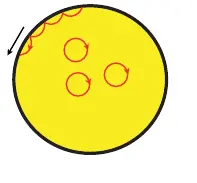
In presence of magnetic field, electrons follow circular trajectories called cyclotron orbits.

• The charged particles can only occupy orbits with discrete energy values, called Landau levels.

• The Landau levels are degenerate, with the number of electrons per level directly proportional to the strength of the applied magnetic field.

• Landau quantization is directly responsible for oscillations in electronic properties of materials as a function of the applied magnetic field.

Now lets look at the mathematical derivation of the above statement. Consider our previous model of two-dimensional electron gas system, say with charge q confined to an area A = \(L_{x}L_{y}\) in the x-y plane. Let the magnetic field applied be \(\hat{B}=B_{z}\hat{z}\) .

Now the Hamiltonian of such a system will be given by

where \(\hat{p}\) is the canonical momentum operator and \(\hat{A}\) is the electromagnetic vector potential.

There is some gauge freedom in the choice of vector potential for a given magnetic field which means that adding the gradient of a scalar field to \(\hat{A}\) changes the overall phase of the wave function by an amount corresponding to the scalar field. But physical properties are not influenced by the specific choice of gauge. For simplicity in calculation, lets choose the Landau gauge, which is

The operator \(\hat{p}_{y}\) commutes with this Hamiltonian, since the operator \(\hat{y}\) is absent by the choice of gauge. Thus the operator \(\hat{p}_{y}\) can be replaced by its eigenvalue \(k_{y}\).

The Hamiltonian can also be written more simply by noting that the cyclotron frequency is \(\omega_{c}=\frac{qB}{mc}\), giving

. This is the Hamiltonian one would encounter for the quantum harmonic oscillator problem as well, except with the minimum of the potential shifted in coordinate space by

.

To find the energies, note that translating the harmonic oscillator potential does not affect the energies. The energies of this system are thus identical to those of the standard quantum harmonic oscillator,

. The energy does not depend on the quantum number \(k_{y}\), so there will be degeneracy.

With this argument we can conclude that the state of the electron can uniquely determined by two by two quantum numbers, n and \(k_{y}\). Now let us focus on the degeneracy of Landau level.

Degeneracy of Landau levels[6,2]¶

Each set of wave functions with the same value of n is called a Landau level. Effects of Landau levels are only observed when the mean thermal energy is smaller than the energy level separation, \(kT << \hbar \omega_c\), meaning low temperatures and strong magnetic fields.

Each Landau level is degenerate because of the second quantum number \(k_{y}\), which can take the values \({\displaystyle k_{y}={\frac{2\pi N}{L_{y}}}}\), where N is an integer.

The allowed values of N are further restricted by the condition that the center of force of the oscillator, \(x_{0}\), must physically lie within the system, \(0\le x0<L_{x}\). This gives the following range for N,

For particles with charge \(q=Ze\), the upper bound on N can be simply written as a ratio of fluxes,

where \(\Phi_{0}=hc/e\) is the fundamental quantum of flux and \(\Phi=BA\) is the flux through the system (with area \(A=L_{x}L_{y}\)).

Thus, for particles with spin S, the maximum number D of particles per Landau level is

Edge modes[4]¶

So far we have discussed the ideal 2DEG scenario. The real samples, though comparatively clean, do not have the transnational invariance that makes each state in a given Landau level have exactly the same energy. Hence there is some sort of broadening of the Landau level. So what is the explanation in this case ?

The initial attempts to explain the effect focused on this effect of disorder, and found that, while two-dimensional electron systems with disorder generally have localized states, this is modified in a magnetic field. Here, the centers of the Landau orbits slowly precess (in opposite senses) around either local minima or local maxima of the potential, corresponding to localized states, but there is an energy at the center of the broadened Landau level at which the centers of the orbits move along open snakelike paths, and the states at that energy are extended as opposed to localized. These edge states act as skipping orbits that precess around the boundary of the system in the opposite sense to that of the Landau orbits, when a particle in a Landau orbit intersects the boundary, and bounces off it.

[1]:”Wikipedia Entry on Hall Effect”, En.Wikipedia.org (Retrieved 25 April 2019).

[2]:”Wikipedia Entry on Landau quantization”, En.Wikipedia.org (Retrieved 26 April 2019).

[3]:”NPTEL :: Physics - NOC: Advanced Condensed matter physics” (Retrieved 27 April 2019).

[4]:F. Duncan M. Haldane, “Nobel Lecture: Topological quantum matter”, Rev. Mod. Phys. 89 (2017), pp. 040502.

[5]:P Sharvari Kulkarni, “Report on Quantum Hall Effect” (April 18, 2019).

[6]:David Tong, Lectures on the Quantum Hall Effect ().

[7]:T. Ando; Y. Matsumoto; Y. Uemura, “Theory of Hall effect in a two-dimensional electron system”, Journal of the Physical Society of Japan 39, 2 (), pp. 279—288.

[8]:Klaus von Klitzing, Benoît Douçot, Vincent Pasquier, Bertrand Duplantier, Vincent Rivasseau, The Quantum Hall Effect vol. 45, (Birkhäuser Basel, ).