Getting to know the cryostat¶

A cryostat is a device used to maintain low cryogenic temperatures of samples or devices mounted within the cryostat. The temperature range can be as low as few milli-kelvin in Dilution refrigerators. Most common ones are either liquid Helium based which can cool to below 10 K or are liquid Nitrogen based, which can cool to about 80 K which is Nitrogen’s boiling point. The sample is mounted on something called as the probe, which houses electrical wires connecting the sample to the instruments used for various measurements. Cryostats can be closed cycle ones, or continuous flow systems. In closed cycle cryostat the cold cryogen (refrigerant) is pumped to the sample chamber and the warm cryogen is extracted and cooled and then recycled into the system. Continuous-flow cryostats are cooled by liquid cryogens from a storage dewar. As the cryogen boils within the cryostat, it is continuously replenished by a steady flow from the storage dewar.

The cryostat at Superconductivity Lab, NISER, for which I had to develop the probe tip, is a customised closed system cryostat provided by ColdEdge. The key features of this cryostat is large sample space and fast cooling. In the large sample space (aka sample well), helium gas is purged (at <0.5 psi pressure) which cools the sample by convection cooling methods. The helium gas is provided from an external gas cylinder. A 0.5 psi relief valve is present for safety in case the sample space becomes over pressurised.

The cooling part of the system is called cold head. It removes heat from the compressors incoming gas by expansion through an internal displacer. The displacer is filled with regenerative material that also helps with the cooling of the gas.

The compressor is part of the cryo-cooler system which cycles helium gas to and from the cold head. It contains an absorber which is used to filter out impurities from the gas which may cause cool down problems for the cold head.

The sample space is attached directly to the cold head and achieves the temperature range (4 - 325K) of the cold head. The sample is attached to the probe which is plunged into cold helium gas inside the sample well. Since the interface remains cold and the probe stick can be removed from the cold interface without having to warm up and break vacuum, different samples can be examined quickly.

By default, the cryostat comes with two Cernox temperature sensors, one for the cold head and the other on the probe to measure sample temperature. Cernox is the best suitable sensor for such low temperature high magnetic field regions.

A vacuum jacket (aka vacuum shroud) is placed over the Cold Head and sample well, which acts as an insulator between the Cold Head and ambient room temperature. It will ensure that ice does not build up on the cooler. Power to the cold head is supplied through the compressor.

A load lock above the sample space, helps to insert the probe without having to warm up and break vacuum of sample space.

It is best to control the heater using the Cernox sensor on the outside of the well rather than using the Cernox sensor on the sample stick. Uniformly heating the outside of the well and adjusting the set point relative to the stick sensor will be much easier than trying to compensate for the convection currents internally in the well.

Design and Fabrication of Probe¶

Design¶

The probe design was made keeping in mind thermal equilibrium of sample and temperature sensor and to maximize the number of connections one can make in a sample. The company for the cryostat had given us a basic stick support structure for the dipstick, which looks like Fig1

The lower end of this structure has a temperature sensor and a heater, so a probe tip had to be designed that can do measurements efficiently.

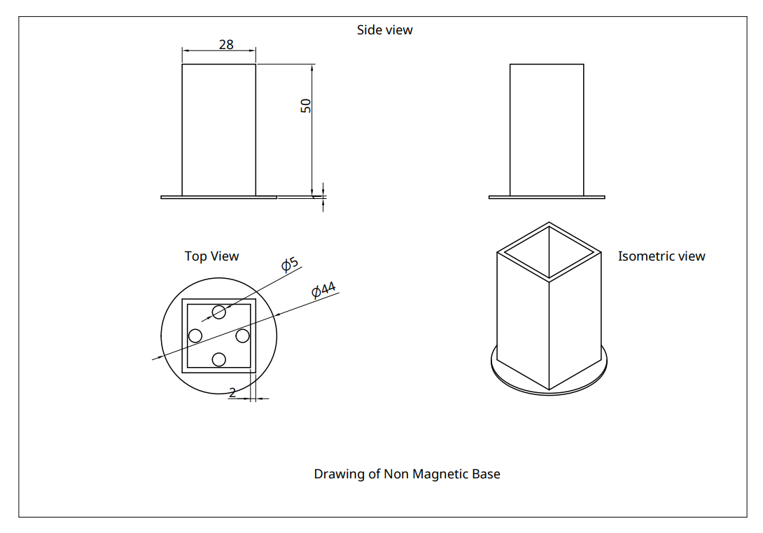
The design finalized is as shown in Fig2. In this design, the brown square part is the copper sheet, the green sheet is an RC filter for all the input wires, and the sample is the purple one, the sample holder pcb can be connected and disconnected to the RC filter PCB, this is so that the sample holder can be removed and taken to the wire bonder etc. There are two versions of this support, the magnetic base (aka flat base)and the non magnetic base (aka square base). In both the case, the 10 pins of each side are connected in parallel. Hence in one go, one can measure at most 10 pads or 4 (2) samples.

Next we had to design the PCB which included an RC low pass filter and a sample holder, the design which was finalised is shown in Fig3 it was designed using a free online service called www.easyeda.com . The RC filter parameters are \(f_c\) = 1000Hz, R=150 ohm, C = 10 \(\mu\) F.

Another version of the square support is the flat support which supports  using magnetic coils for magnetic measurements is as shown in fig3

The RC filter works by using capacitor and resistor to attenuate high frequency noise. A circuit diagram for the same can be seen in Fig 5. The characteristic bode plot expected for a functioning RC filter is shown in Fig 6.

Fabrication¶

The pcbs were designed and then sent to www.jlcpcb.com for fabrication of PCB. The electronic components required for the board were ordered from www.lcsc.com.

The delivered product is shown in Fig 7.

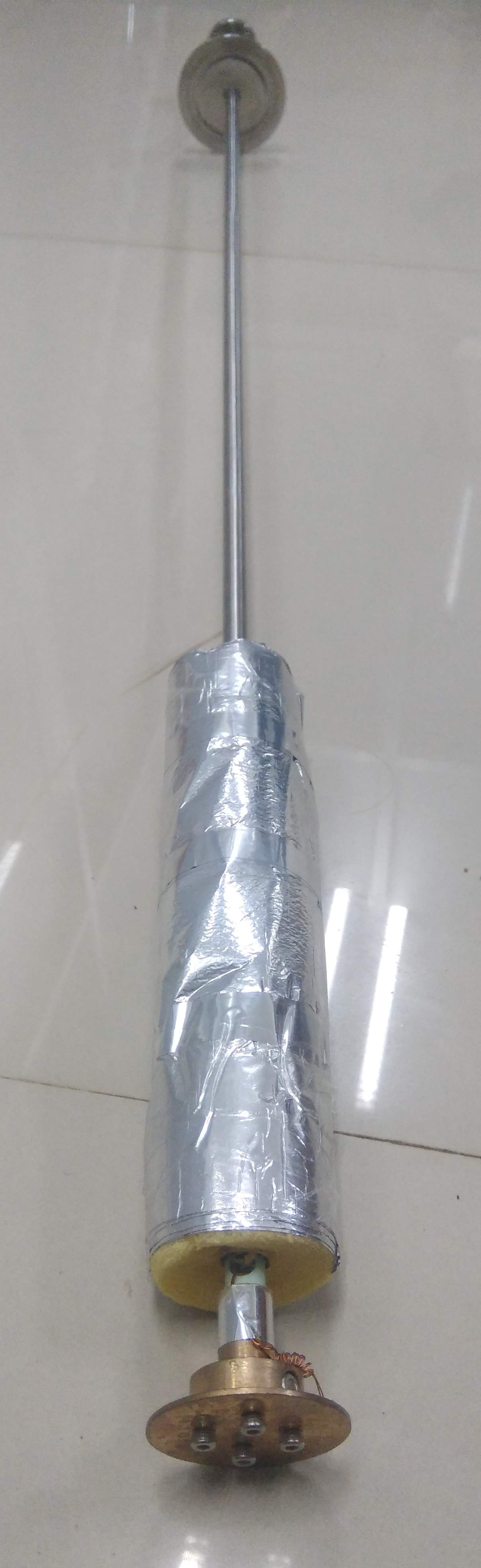
The base was made in house using copper sheets which were cut using an angle grinder to the required measurements. The joints were fixed by brazing it with copper. The finished probe ends are seen in Fig 8.

For measurement purpose, a sample of sputtered Nb thin film (55nm) was stuck on the copper base of the holder and wire bonding was done in 4 probe arrangement. The sample after wire-bonding is in fig8 .

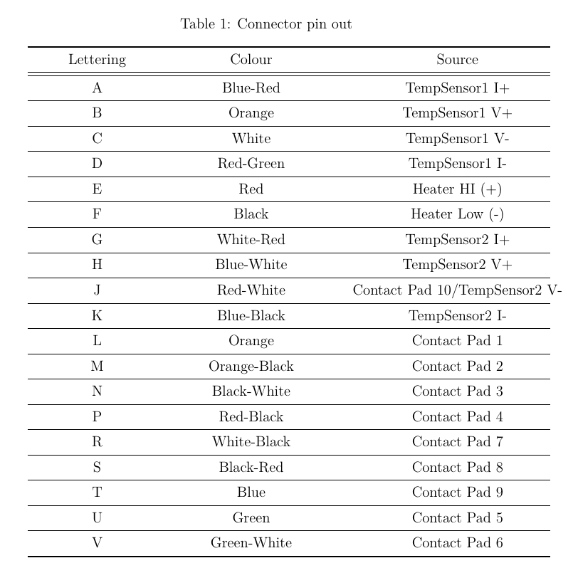
The wiring for the probes were made with 37 gauge enameled copper wire twisted in pairs (Fig 9). The pin out for the connector can be found in Table 1.

The pads of the sample are connected to the break out box (fig 22).

Software for data acquisition¶

The signal from the sample is fed into the temperature controller and Source meter unit. The data from these instruments is gathered using a software written in Labview. A schematic of data flow is in Fig10.

All the software tools required for data acquisition is compiled into a Labview project file “MeasurementLibrary.lvproj”. A shortcut to this file is kept in desktop (Fig 11).

When the project file is opened, A list of all the available programs is shown (Fig 12)

This software suite consists of

• 4 probe resistance measurement interface (“B2912A_4probe_ohms.vi”)

• Basic GPIB communication tester (“basic_gpib_write_and_read.vi”)

• LS336 Heater Output Configuration Panel (“LS336 Configure Heater Output Control Parameters and Acquire Single Reading.vi”)

• LS336 Temperature Logger (“LS336_read_2temperature.vi”)

• Basic RT,Tt Plotter (“Plot_RT_Graph.vi” and “Plot_Tvst.vi”)

• RT Logger with Temperature controller (“RT_measurement.vi”)

Let us look at the functioning of each program one by one.

4 probe resistance measurement interface¶

The 4 probe resistance measurement interface is shown in Fig 13.

The software takes in the SMU VISA name (hardware address) and all the resistance measurement mode settings and does a single measurement. The hardware address for LS336 is GPIB0::1::INSTR and that for the SMU is GPIB0::2::INSTR (or USB:xxxx in case it is connected via serial).

Note: If you change some parameter, when you close the program there might be a confirmation to save changes (Like Fig 14.)

ALWAYS CLICK “DONT SAVE ALL”, this is to ensure no pre-configured parameter gets changed by accident.

Basic GPIB communication tester¶

The interface for Basic GPIB communication tester is shown in Fig 15.

This tool allows you to debug GPIB connections and to check the state of the instrument. After selecting the right Hardware address, (VISA Resource name) you can write any serial SCPI commands in the Write buffer and when you execute the program the instruments response is shown in read buffer. Typical serial SCPI commands include:

\*IDN? - Identify \*RST - Reset \*OPC? - Operation complete query \*CLS - Clear Status

.

LS336 Heater Output Configuration Panel¶

The interface for LS336 Heater Output Configuration Panel is shown in Fig 16.

This software initializes the instrument, allows the user to determine if heater output control parameters and setpoint values are sent, takes a single sensor reading, and then closes the instrument.

LS336 Temperature Logger¶

The interface for LS336 Temperature Logger is shown in Fig 17.

This software logs the sensor reading (of two inputs), and then saves the data in a tab separated file specified by the user.

Basic RT,Tt Plotter¶

The interface for Basic RT,Tt Plotter is shown in Fig 18.

The application takes in a tab separated text file containing data of index,V,I,R,\(T_(coldhead)\),\(T_(sample)\) (obtained from temperature logger or RT Logger with Temperature controller )and then plots the RT , Tt graphs with T being the \(T_(sample)\) .

RT Logger with Temperature controller¶

The interface for RT Logger with Temperature controller is shown in Fig 19.

This application is basically all the above utilities put in one. There are two tabs, one for controls, the other for viewing the plots. In the control tab, one can set the parameters for SMU as well as Temperature controller. When the application is executed with the correct parameters set, the data of index,V,I,R,\(T_(coldhead)\),\(T_(sample)\) are stored in a tab separated text file at user specified location. The controls on the temperature controller side might look daunting at first, however a quick glance of LS336 manual clears up all the parameters.

List of procedures¶

Cryostat connections.¶

The connections of Vacuum jacket, Vacuum pump, Pirani gauge, load lock and the valves can be made as shown in Fig 20.

The temperature sensor connections are to be made as in Fig 21. The temperature sensor on the probe needs to be connected to Input B and that of the Cold Head to Input C (This is needed as the proper curves are chosen for this particular arrangement). The heater on the probe needs to be connected to Output 2 (50W) and that of the Cold head to Output 1(100W). Both the heaters are 50 Ohm heaters.

The break out for the pads on the sample holder can be accessed through the break out box (Fig 22.)

Each wire from the Hermetic connector is colour coded (as in Fig 23), the pin-out for the same is in Table .

NOTE: Never create vacuum in sample space, the rubber bellows can get torn under vacuum.

Check connections for leaks.¶

• After making the connections,vacuum the vacuum pipe( turn off the Load Lock Valve ,turn on the Pirani Gauge). now slowly turn on the Vacuum Valve and . Wait till 10E-3 Torr of vacuum is achieved.

• Spray all joints with Isopropanol and watch for a spike in vacuum. If spraying Isopropanol over any joint causes a spike in vacuum, you know that you have a small leak. Re-grease 0- rings and recheck. Any debris on the O-ring or inside the O-ring groove will certainly cause a leak path and will be noticeable .

Purging the Interface.¶

Before turning the system on (after a long gap) you will need to purge the interface to remove any air that is trapped inside the sample well. This step is not required in regular use. This step can also help in getting a clear view through view port ( Fig 24) by removing some condensation.

• Supply about \~0.5 psi of pressure to the gas inlet of the cryostat through the regulator. (NOTE: Supplying more than 20 psi to the Regulator may cause damage to the internal diaphragm. )

NOTE: If the sample well is not free of moisture and/or air it will cause the gas inlet tube to freeze below liquid Nitrogen temperatures. When this occurs the sample well will start to create vacuum and will suck the bellows into the well, potentially ripping or forcing the bellows from it’s clamp.

Starting the system (Cool Down).¶

• Turn on the water cooler (set at 15 degree Celsius) 30 minutes before hand.

You can check if the cooler is turned on or not by feeling vibration of water moving through the pipe.

After few minutes both the pipes should feel cold to touch.

• Make sure that there is no leak in any connections.

• Turn the gas regulator to about 10psi.

• Make sure that He is flowing in the sample chamber.

• Turn On the compressor.

Once the compressor is turned on, you will hear the Cryocooler begin to start pumping. The Cryocooler will take approximately 120 minutes to cool down.

Now that the Cryocooler is running, maintaining the 0.5 psi pressure on the sample well will be critical for the sample to reach minimum temperature. If the cryostat is not able to reach its desired temperature then one of the reason can be empty cylinder. As the cooler gets colder it gets denser and falls to the bottom of the well. The interface will pull more gas into the system as it cools for this reason. Make sure the external gas cylinder has enough helium to supply the system with gas throughout the entire run.

Sample Insertion.¶

• Replace the shipping cap with the quick clamp .

• Release the load Lock

• Loosen the gripper of the probe and slowly push the probe towards the cold end.

• Make sure to push the probe in steps of 75 K so that no thermal shock is offered to the sample or probe.

• Move only until the mark made by paper clip (\~34 inch above the tip of the probe). This is the point where the probe is just above the cold head.

Changing a sample.¶

Keep in mind that when changing the sample it is imperative to block out as much air from getting into the sample well as possible. Remember you have slightly positive pressure, so this will help keep air out.

No warm up of the system is needed during change of sample.

• Loosen the gripper of the probe and slowly pull the probe towards the hot end.

• Make sure to pull the probe in steps of 75 K so that no thermal shock is offered to the sample or probe.

• Once the probe is above the load lock, close the load lock.

• Use the LS 336 to heat up the coil on the probe to bring it to 300K (only do this after the probe gets to 280K or above).

• Once the temperature sensor on the probe reads about 300K, open the quick clamp to remove the probe.

• Replace the quick clamp along with the shipping cap.

Shut down.¶

Once the experiment cycle is done or there is a requirement of shutdown for maintenance the following procedure may be followed:

• Allow the cold head to warm up on its own. Opening the vacuum while the system is still cold will cause it to ice up, potentially damaging the sensors.

• Once it warms above 200K, you may then open the vacuum,.

• For faster warm up, you can use the temperature controller to heat the system up to room temperature. If you decide to heat the system up like this, again, make sure the Cryocooler is running at all times. Allow the heat to stabilize for 15 or 20 minutes at room temperature then shut the temperature controller down along with the Cryocooler.

• Maintain small gas purge on the sample well while the system is warming to room temperature. This will assure that moisture does not collect inside the well.

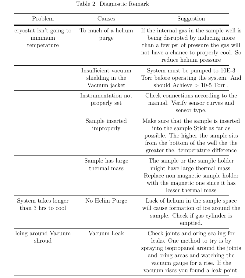
Diagnostic remark¶

Measurement Results¶

One of the very first measurement done was of the RC filter, which was tested using Analog Discovery 2 and the data is as in Fig28 and one can easily conclude that the RC filter was working as intended at the cut off of 1000Hz at room temperature.

It was suspected that the resistor and capacitors might not work reliably at low temperatures (since the resistor is made from thin film of a metal oxide and the capacitor is made of ceramic material). In order to test it, a resistor was mounted on a puck (Fig 29)and a RT graph was drawn using a PPMS made by Cryogenic Ltd which was present in the lab.

The results showed minimal change of resistance at low temperature (160 ohms at below 10 K). Hence the smd resistor worked fine at low temperatures. The cryogenic PPMS didnt have ready method to measure capacitance as a function of temperature. Hence this measurement was only possible after assembling the PCB and mounting it on the probe. This exercise revealed that the capacitance dropped to 10 nF below temperatures of 10 K and an RC plot showed the cut off frequency shift to 100KHz. Nullifying the use case of the RC filter. The bode plot for this trial is in Fig. 30

Finally, one trail to measure the superconducting transition of a 55nm thin-film of Nb was done using the probe.

The RT graph of the Nb sample as obtained is as in Fig 31. From this graph we can conclude that the Tc for the given sample is 7.68 K.

An attempt was made to fabricate a Nb|\(Nb_2O_5\)|Nb Josephson Junction and to measure the IV graph of the same. The junction was made by taking two strands of Nb wire (50 \(\mu\) M thick ) cleaned with 0.5 molar HCl. One strand was oxidized at 100 degree Celsius for a fixed time, and then the two wires were made to contact each other under tension provided by a stick with sharp edge (Fig 32). However not much success was found.

Conclusions¶

The probe was successfully fabricated according to the initial design. However many new modifications come into mind after going through the 2 month process. The first major draw back was the failure of the RC filter, which was caused by the SMD capacitor, one can modify the circuit for an inductor instead of capacitor, or one can replace the current SMD capacitor with a different class capacitor. The second draw back was the large thermal mass of the non magnetic base. To counter this, one can reduce the number of samples, thickness of Copper, Increase joint thermal conductivity (by applying thermal paste or indium sheet). Thirdly, the size of the probe is very close to the allowed limits of the system, hence a new design can have a smaller sample holder and adapter. Next, the problem of ease of changing adapter has to be addressed by modifying the entire design . One can also think of replacing the default shielding that the probe comes in with something like silica aerogel for better insulation. One of the major problem faced was that the Helium cylinder gets emptied very quickly, this can be because of helium escaping through the plastic tubing, one can fix this by replacing the tube with cooper piping. Also, PID values for both the heater have to be optimised, the current values of 10,20,10 give a moderately good result. Finally the LabVIEW program can be made more robust, the current program is as basic as it can get, more features such as automation of multiple trials using some form of sequence editor can be thought of.

A pdf version of this page (with better formatting) is available here. And the LabVIEW software mentioned in the article is available here