Introduction¶

This article is an adaptation of my Masters thesis report ( second semesters ), where I worked on the modelling and simuation of Josephson Junctions. All the codes and data used in this article can be found in the github repository. The previous article talked about the the fabrications of Josephson Junctions and their charecterisation ( first semester ). At the beginning of this thesis, we introduce basic theoretical concepts that underlay the device we are trying to study, i.e. the Josephson Junction (JJ). The theorey of superconductivity was breifly described in the previous article. We first look at the Josephson effect, which describes the physics of a Superconductor-Insulator-Superconductor sandwich and then look at a popular model of a realistic Josephson junction, namely the RCSJ model. Later we will try to understand various aspects of fabrication and characterisation of such devices.

Josephson Junctions¶

Prior to 1962, researchers were familiar with quantum mechanical tunneling of normal electrons through a weak barrier; however, the probability of tunneling of a cooper pair was thought to be insignificant given that the pair as a whole would have to tunnel through the barrier. In 1962 Brian David Josephson showed that this tunneling probability is not low as previously thought. He predicted theoretically that two superconductors that are coupled (are in close proximity) by a weak link, which link may be made of a normal metal, an insulator, or a constriction of superconductivity, can still let the super current flow through them (Josephson 1962). This macroscopic phenomenon was given the name Josephson effect.

Josephson demonstrated that, for a short junction, the current that flows through the junction when no voltage bias is applied, and the phase difference \(\phi\) across the junction, which is the difference in the phase factor between the order parameter of the two superconductors, are related through the relation:

Here, \(I_{c}\) is the super current amplitude and \(\delta=\phi_{1}-\phi_{2}\) , where \(\phi_{i}\) is the phase of each superconductor. This phenomenon is known as the DC Josephson effect. Josephson also showed AC Josephson effect where an applied constant voltage bias V on the junction leads to sinusoidal oscillations in the junction current and is governed by the equation:

where \(\Phi_{0}\approx2\times10^{-15}\) Weber is the flux quantum.

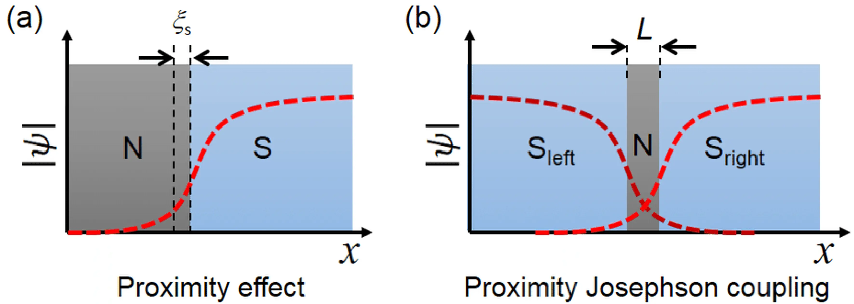
The DC Josephson effect is explained by a process known as Andreev reflection (Schrieffer and Tinkham 1999). A.F.Andreev explained the phenomenon in 1964 establishing the concept of the so-called Andreev reflection This reflection occurs at the interfaces between the superconductor S and a normal metal N. Andreev suggested that an electron that approaches the interface from the normal metal side can travel through the superconductor side by the formation of a Cooper pair with another electron with opposite momentum and spin on the superconductor side. At the same time, reflect a hole inside the normal metal region thus balancing the charge. As a result of this cycle, a pair of correlated electrons is transferred from one superconductor to another, creating a super current flow across the junction. It explains how a normal current in the normal metal side becomes a super current in the superconductor side. The AC Josephson relation in essence suggests that a Josephson junction can be a perfect voltage-to-frequency converter. The inverse is also possible by using a microwave frequency to induce a DC voltage in a Josephson junction, this phenomena is known as inverse AC Josephson effect.

RCSJ model¶

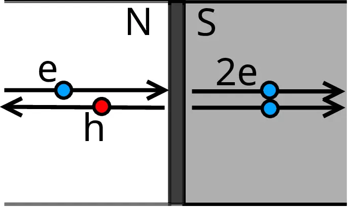
A Josephson junction, is typically composed of two superconducting electrodes separated by weaklink which is typically insulating, thus such a junction would have some unavoidable capacitance \(C\) (Just like the parallel plate capacitor separated by a dielectric). If the junction current exceeds the critical current of the junction then quasi-particle excitations are generated. These quasi-particle currents are not superconducting and can be quite lossy just like a normal metal current, so we represent this as a normal resistor \(R\). This gives us the resistively and capacitivly shunted junction (RCSJ) model. This model helps us simulate the characteristics of a Josephson junction. A schematic representation of the same can be seen in Fig 1.

Writing out Kirchov’s circuit laws for the RCSJ model (from Fig 1.)we can find

or

Rearranging as

we can interpret Eq [eq:dammpedeqn] as the dynamics of a damped particle with the following physical properties:

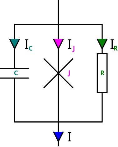
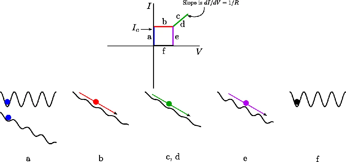
The dynamics of the Josephson junction phase difference in-terms of the damped particle can be described as follows: (Fig 2)

• The junction has a simple cosine potential when there is no junction current (at I=0). At this point, the pseudo-particle is caught in one of the cosine’s wells, as shown in Fig 2a. We can observe the effect of an extra linear term to the potential as we introduce some current. Because the potential now resembles a tilted washboard, it’s known as the tilted washboard potential. There are still vallies in the potential if the bias current is less than \(I_{c}\), and the ball remains stuck, as shown in. Fig 2a. Because the junction phase (i.e the pseudo-particle) is stuck at a fixed value of \(\delta\), the voltage is zero (as \(V\propto\dot{\delta}\) ). As demonstrated by the horizontal blue line, this is the section of the IV curve where an increase in junction current does not result in an increase in junction voltage. Because the junction element is still superconducting, all current flows through the tunnel element and none through the resistor at this point, resulting in the junction.

• As the current is increased past \(I_{c}\), the linear term in the potential begins to dominate the cosine part, and the vallies fade away. As demonstrated in Fig 2b the junction pseudo particle then rolls downhill. The pseudo particle is now in a time-varying phase, and the junction voltage is non-zero and approaches a finite value, as shown by the red line in Fig 2b

• Because the current I now exceeds the tunneling element’s critical current, the tunneling element no longer acts as a superconductor. The formation of quasi-particles makes the connection resistant. In other words, the resistive element carries practically all of the current. Further increases in current result in a linear increase in voltage, identical to that of a typical metal, as indicated by \(V=IR\), as shown in Fig 2c, and by the green line marked Fig 2c.

• As the current is reduced, we return to the green line, as shown by the mark Fig 2d. The rest of the process depends on how fast we are raising and lowering the current. The potential regains its cosine nature and regains vallies, as we lower the current below \(I_{c}\) .

• If there were no dissipative forces as is the case when we sweep fast enough or when whatever dissipation remains can’t completely stop the particle, the particle would continue to roll down as it already has energy. Therefore, even as I is lowered below \(I_{c}\) we still have time varying \(\delta\) and therefore still have a measurable voltage. This can be concluded from Fig 2e and the pink line in Fig 2e

• In the end, we go back to no bias case where the potential is again a cosine term and as we slowly sweep the voltage we slow down and finally stop the particle. Then as we increase the negative bias the process starts all over in reverse.

Josephson Junctions in the Presence of a Magnetic Field¶

In Eq[eq:JJ1] we saw that he Josephson Junction current depends on the phase difference \(\delta\) across the junction. When an external magnetic field is applied, the field influences the phase difference \(\delta\), this in turn causes interesting dynamics between the Josephson Junction current and the applied external magnetic fields. It can be shown that in the case of a small Josephson Junction this dependence follows the relation(Schrieffer and Tinkham 1999):

here \(\Phi_{J}=\mu_{0}Hw(d+\lambda_{1}+\lambda_{2})\text{ is the magnetic flux linked to the whole barrier }\)with \(w\) being the width of the barrier, \(d\) the barrier thickness, \(\lambda_{1},\lambda_{2},\)the penetration depths of the two superconductors. This behavior was first experimentally found by Rodwel (Rowell 1963), in a Pb-I-Pb junction at 1.3 K. This is the standard from of the Fraunhofer pattern \(F(x)=I_{0}\sin^{2}(\pi x)/(\pi x)^{2}\)and is seen as a unique characteristic confirmation of a Josephson junctions. This Fraunhofer-like result, which is akin to diffraction of monochromatic, coherent light passing through a slit, provides a validation of the sinusoidal current phase relation (CPR). For a SQUID, the critical current-magnetic field characteristic is similar to that of Josephson Junctions with the addition of SQUID oscillations superimposed on it. Both of these signatures are in the simulations done in the later section. In case of junctions with ferromagnetic behavior, at certain temperature and barrier width, a \(\pi\)junctions could be observed. This is due to exchange field-induced oscillations of the order parameter and is very sensitive to the temperature and the ferromagnetic layer thickness. In such materials the CPR could be written as \(I(\phi)=I_{0}sin(\phi+\pi)\), and doubling of periodicity in \(I_{c}\)vs \(H\) is observed(Frolov et al. 2004). In materials with broken time-reversal and broken parity symmetries (this can be obtained in systems with both a Zeemanfield and a Rashba spin-orbit coupling(Assouline et al. 2019; Strambini et al., n.d.)), the CPR could take the form of \(I(\phi)=I_{0}sin(\phi+\phi_{0})\) (Assouline et al. 2019), in Josephson junctions this term leads to the anomalous phase shift, which could manifest as the presence of second harmonics in the critical current - phase relation (Stoutimore et al. 2018). This system is also simulated as a part of the thesis, where in the \(I_{C}H\) behavior is replaced with the following:

Simulation Details¶

The characteristic signature of a Josephson junction, apart from its current voltage relation (IV) is the Critical current \(I_{c}\)dependence on the applied magnetic field H ( \(I_{C}\)vs H or \(I_{C}H\)).

The PPMS in the lab has builtin recipes only for DC measurement and as such DC measurements like IV are relatively slower (1 IV scan in 10-15 minutes on good resolution). Thus getting data for \(I_{c}H\) would require multiple IVs to be measured at a sweep of magnetic field H. This would take almost a day per device on a decent resolution and thus cant be done frequently. The more easier measurement would be to set and constant current (say the \(Ic\) at zero magnetic field) then measure the Voltage as a function of changing magnetic field ( V vs H or VH ) however, there is little literature regarding the characteristics of VH relation (or magneto resistance ) of a Josephson junction.

Thus the main goal of the thesis is to verify the correlation between the \(I_{C}H\) and \(VH\) signatures of a Josephson junction via simulation. simulation part of the thesis is to first setup the numerical solution to the ODE [eq:dammpedeqn] , then simulate an I - V measurement, Iterate the IV sweep over multiple magnetic fields linearly spaced between \(-2\frac{\phi}{\phi_{0}}\) and \(2\frac{\phi}{\phi_{0}}\) . This would give us the data of all permissible sets junction current \(I_{J},\)junction voltage \(V_{J}\) and the applied magnetic field \(H\) that are the possible states of the given Josephson Junction. Finally, one could correlate the simulation with experimental data for junctions with and without second harmonics from \(I_{c}H\) and \(VH\) measurements. First lets us try to understand the systems ODE.

Modeling the ODE¶

We model the Josephson junction using the RCSJ model as described in sec[subsec:RCSJ-model]:he total current running through the network is

Due to quasiparticle tunnelling, the resistance in reality relies on both the temperature and the voltage across the junction as described by this equation:

where typically \(R_{sg}\gg R_{n}\). The characteristic voltage of the junction is accordingly defined as \(V_{c}=I_{c}R_{n}\).

The current-phase relation (CPR) \(I_{s}(t)=I_{c}\sin(\phi)\) describes the supercurrent via a Josephson junction (JJ), where \(I_{c}\) is the critical current and \(\phi\) is the junction phase-difference. The CPR can be stated in more broad terms as (Pal et al. 2014; Tanaka and Kashiwaya 1997)

, and when the first harmonic is suppressed (for example, at a 0 –\(\pi\) transition)(Sellier et al. 2004), the second harmonic may become apparent. We try to determine the influence of adding a second harmonic CPR in the I c H and V H behavior in this thesis by simulation.

Before we try to solve the ODE [eq:ODE], we can try to simplify the ODE by normalising the equation.

This helps in minimizing the round off errors, for instance if one variable has the value 24582 (units a) the other variable could be in the order 0.001861(units b). The significance of the second variable could be irreversibly lost while executing any operation pertinent to these variables, such as multiplication. One technique to assist limit these possible losses is to normalise the variables first. The equation is simplified with normalized time ( unitless ) via the plasma frequency, \(\tau=\omega_{p}t\) where \(\omega_{p}=\left(2eI_{c0}/\hbar C\right)^{1/2}\):(Schrieffer and Tinkham 1999)

\(\omega_{p}=\frac{1}{\tau_{p}}=\frac{1}{\sqrt{L_{c}C}}=\sqrt{\frac{2eI_{c}}{\hbar C}}\) and \(dt=\frac{1}{\omega_{p}}d\tau\rightarrow\frac{d^{n}}{dt}=\omega_{p}^{n}\frac{d^{n}}{\tau}\), applying these factors we get

In this eq [eq:FinalODE] Q is the damping factor (or quality factor) which depends on the inherent resistive and capacitive components of the RCSJ model. This Q is identical with \(\beta_{c}^{1/2}\), where \(\beta_{c}\) is a frequently used damping parameter that was introduced by Stewart and McCumber. In the case of heavy damping \((Q\ll1)\) we see the same IV behavior for increasing and decreasing current, however in the case of under damped junction (\(Q\gg1)\), while decreasing the current, we see that the junction remains in the non zero voltage range below \(I_{c}\). This behavior is also explored in the simulations.

The \(I_{c}\)in eq [eq:FinalODE], is the critical current and its dependence with magnetic field is to be incorporated separately in the simulation based on Eq [eq: IcH 2].

Simulation parameters¶

The ODE [eq:FinalODE] can be converted to a system of first order ordinary differential equations, and then it can be passed on to a ODE solver like scipy.integrate.odeint with the initial values.

The result one such ODE solve is \(\phi\) and \(\mathring{\phi}\) as a function of time for the given initial conditions of \(\phi\) , \(\mathring{\phi}\) and \(I\). The dynamics of such a system depend vastly on the initial condition given to the ODE. As an example consider the ODE solution as a function of time (in \(\tau\)) for different initial conditions for \(\phi\) and \(\mathring{\phi}\) in Fig 3.

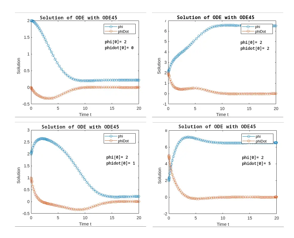
For the first iteration of the simulation (0 current and 0 phase difference) starting point for \(\phi\) and \(\mathring{\phi}\) should be set to zero as any \(\mathring{\phi}\) would have to start from the moment a superconducting phase sets up and gradually evolves with time to reach equilibrium.

After the system evolves for a certain amount of time steps (which needs to be adjusted depending on Q), the voltage is calculated by averaging over the last cycle (detected as a percentage of the entire time solve). If there’s no voltage cycle, the voltage gets set to zero. The initial condition for the next run (next current value in the IV seep) is the final state of that previous one.

The percentage of final cycle and the number of cycles to be run is determined for each range of Q (below 0.1, below 1 below 10, below 100) and kept in a function called timeparams.

The entire process is then iterated over the given range of given currents. It must be noted that since the simulation for current depends on the previous relaxed values for \(\phi\) and \(\mathring{\phi}\), the voltage values for a given I depend on whether the current is a part of the increasing I cycle or decreasing I cycle. Thus one could clearly differentiate between the over damped IV and under damped IV based on the presence of re-trapping current. See fig 4. In the case of heavy damping \((Q\ll1)\) we see the same IV behavior for increasing and decreasing current, however in the case of under damped junction (\(Q\gg1)\), while decreasing the current, we see that the junction remains in the non zero voltage range below \(I_{c}\).

The overall architecture for setting up the simulation including several functions have been referenced from (Schmidt 2017).

Simulation Results¶

After plotting the IV sweeps for various Q as in Fig 4, it was found out that Q value between 1 and 5 has the closest resemblance to experimental IV. Thus all further simulation were made with Q=1.5 and Q=0.5 for checking the over damped and under damped cases.

Plots of the simulations are showing in Fig6 & 8.

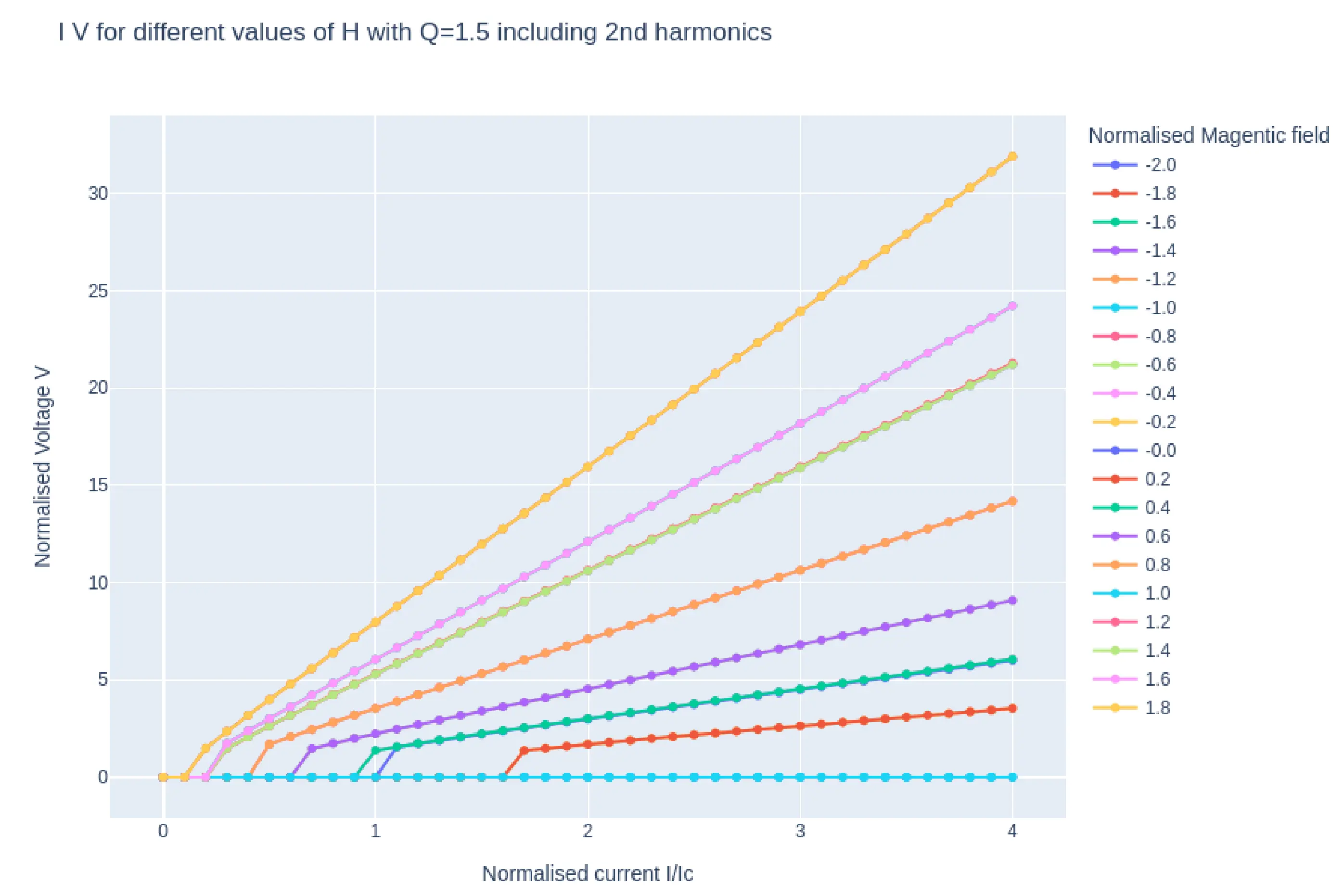
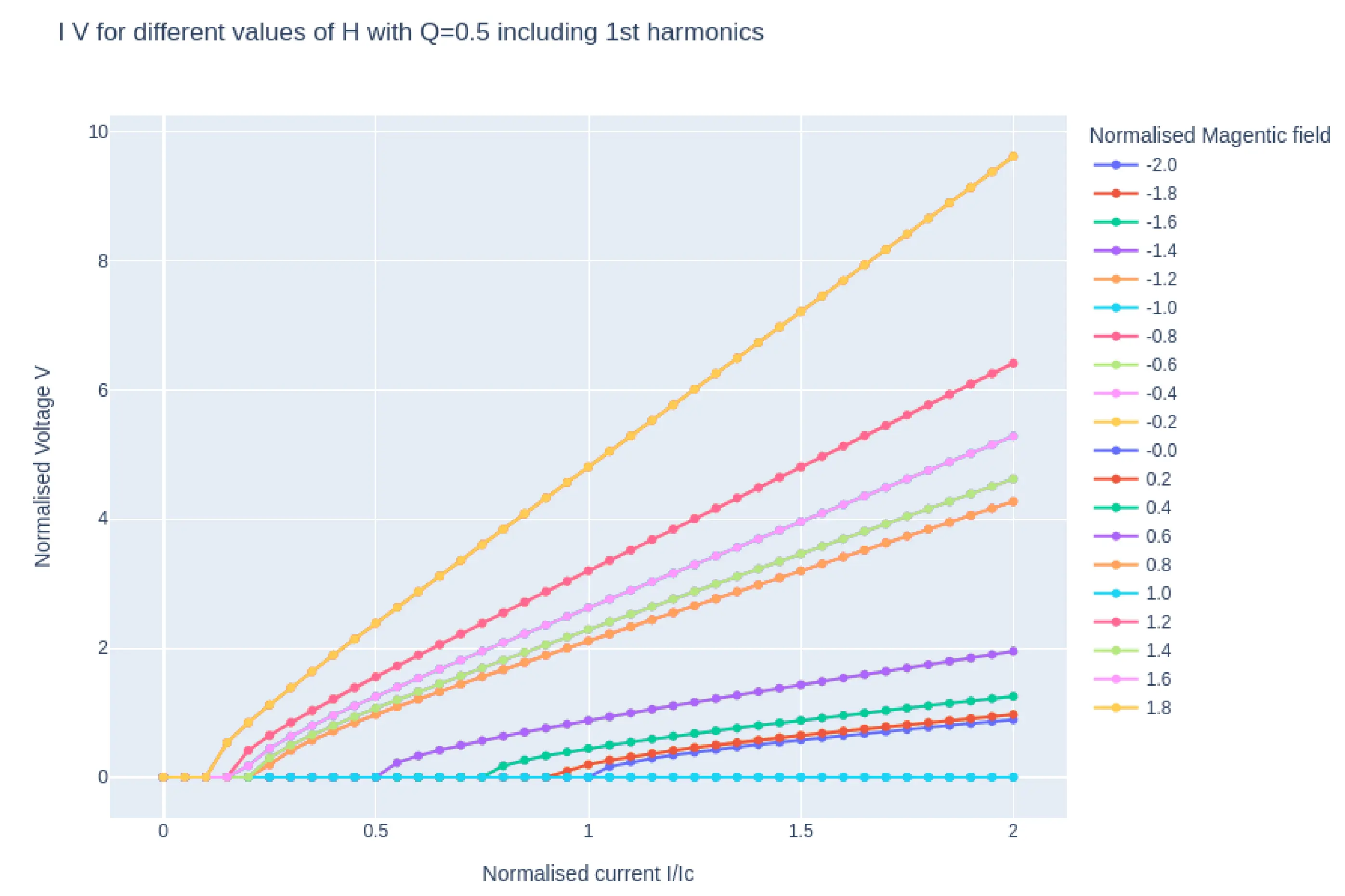
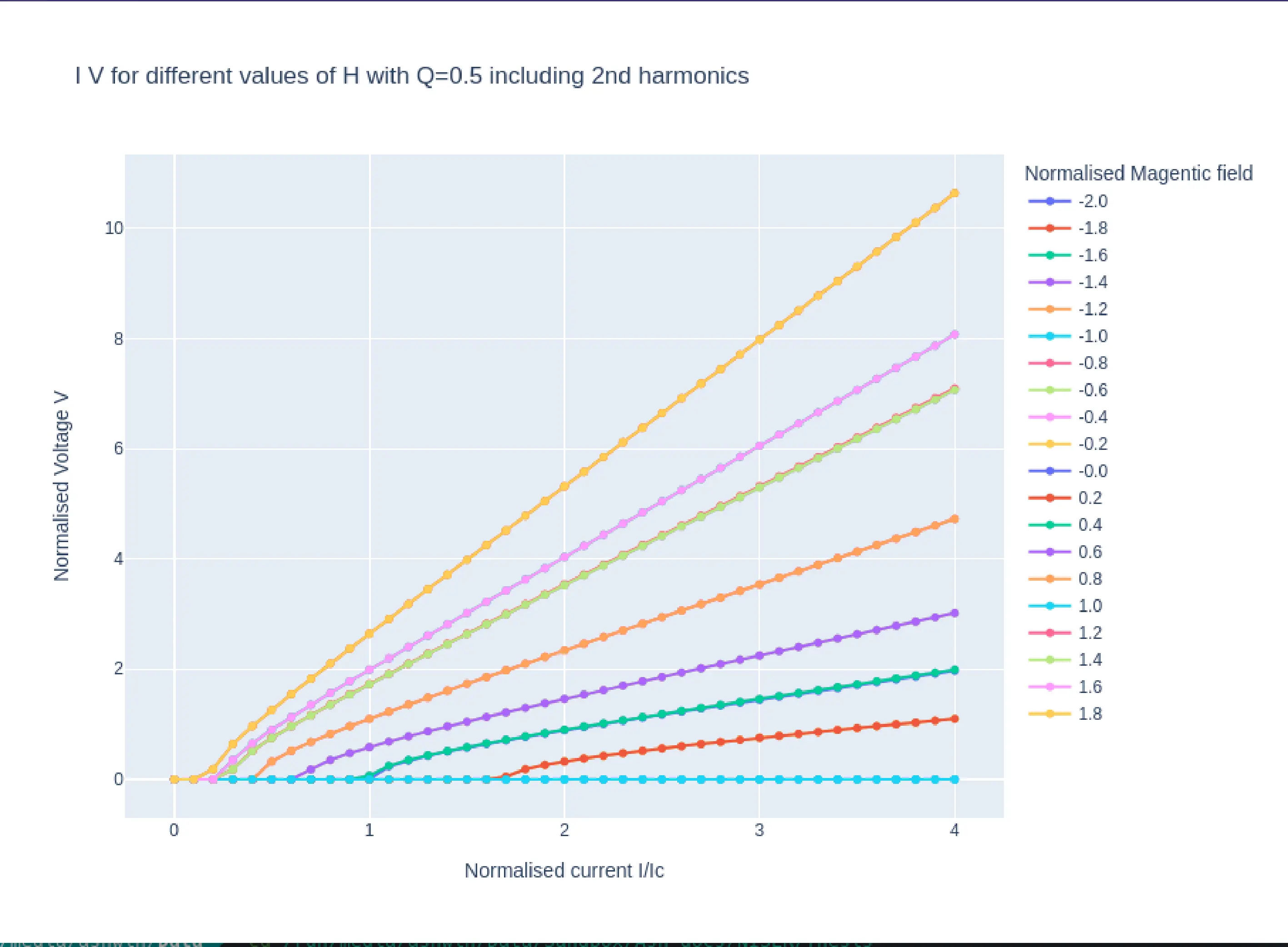
In the case of heavy damping \((Q=0.5)\) we see the same IV behavior for increasing and decreasing current, however in the case of under damped junction (\(Q=1.5)\), while decreasing the current, we see that the junction remains in the non zero voltage range below \(I_{c}\)which is as expected. The variation in the \(I_{c}\)as a function of applied magnetic field \(H\) is also evident.

The next part of the analysis is to compute the \(I_{C}H\) data and \(VH\) data from these simulations in both the first harmonics case as well as the second harmonics case.

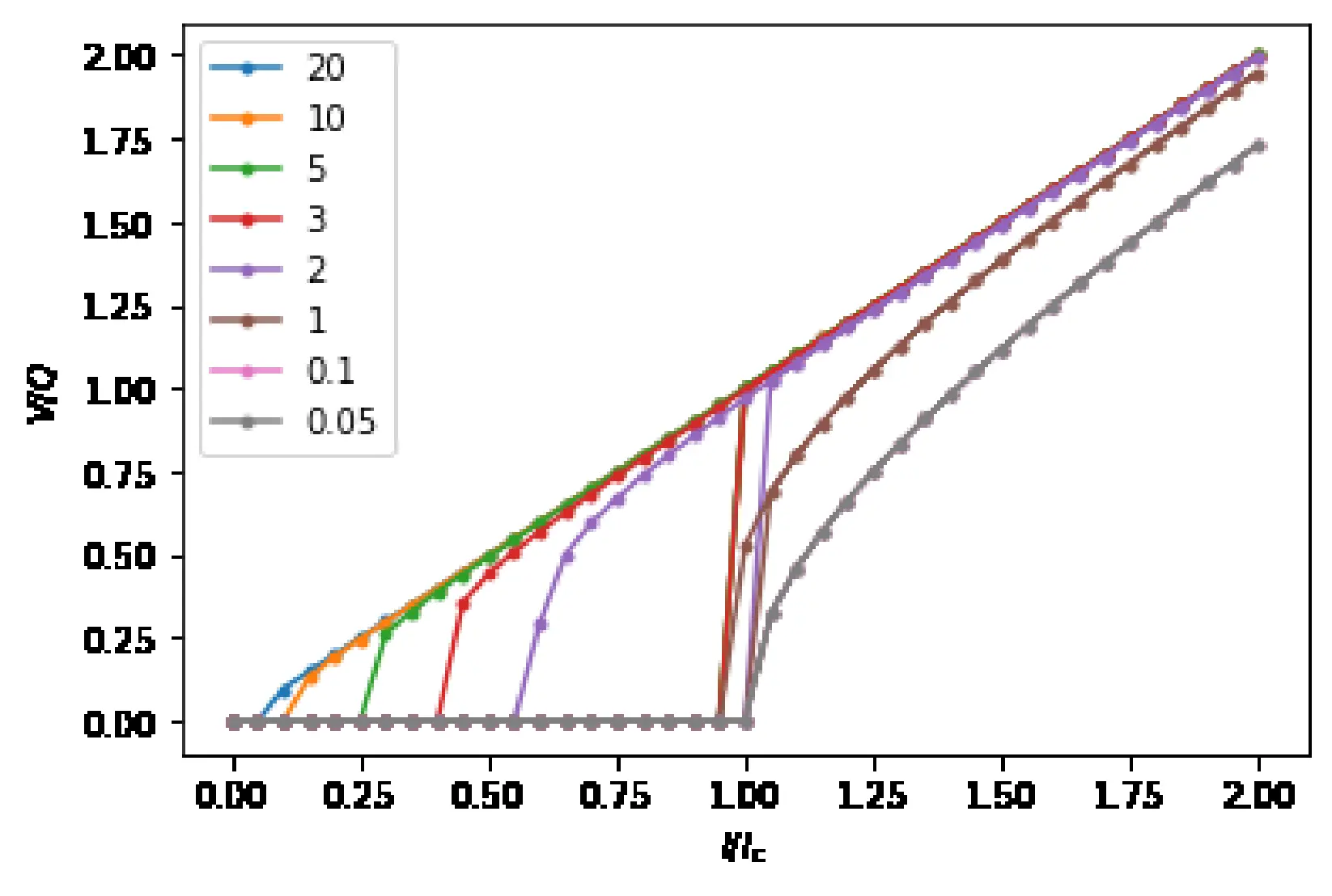
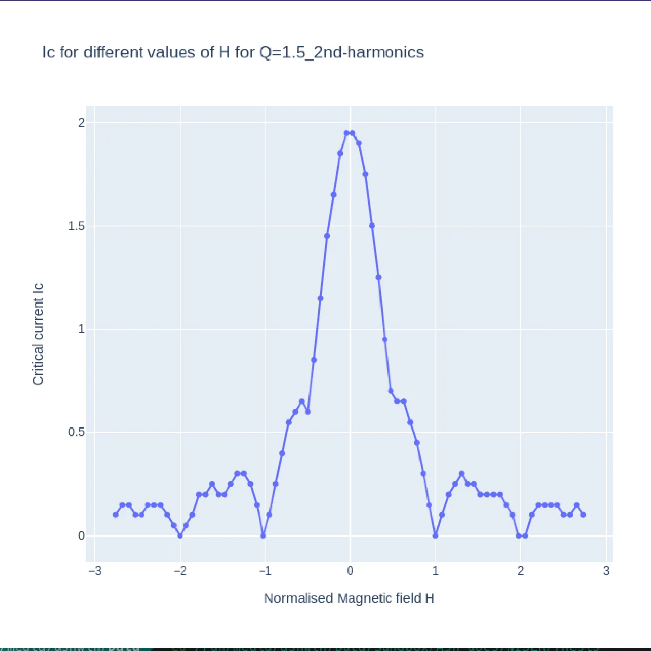
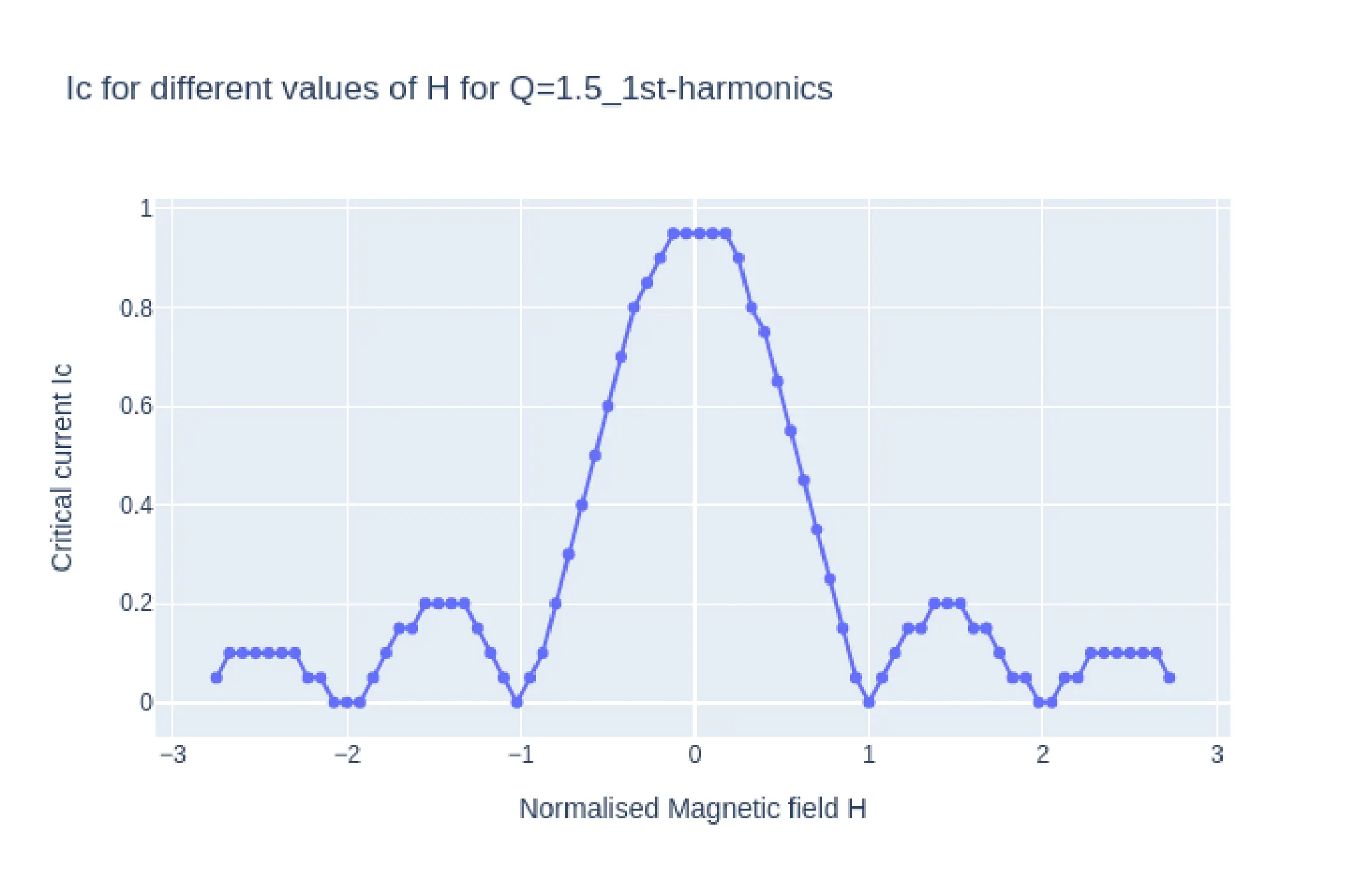
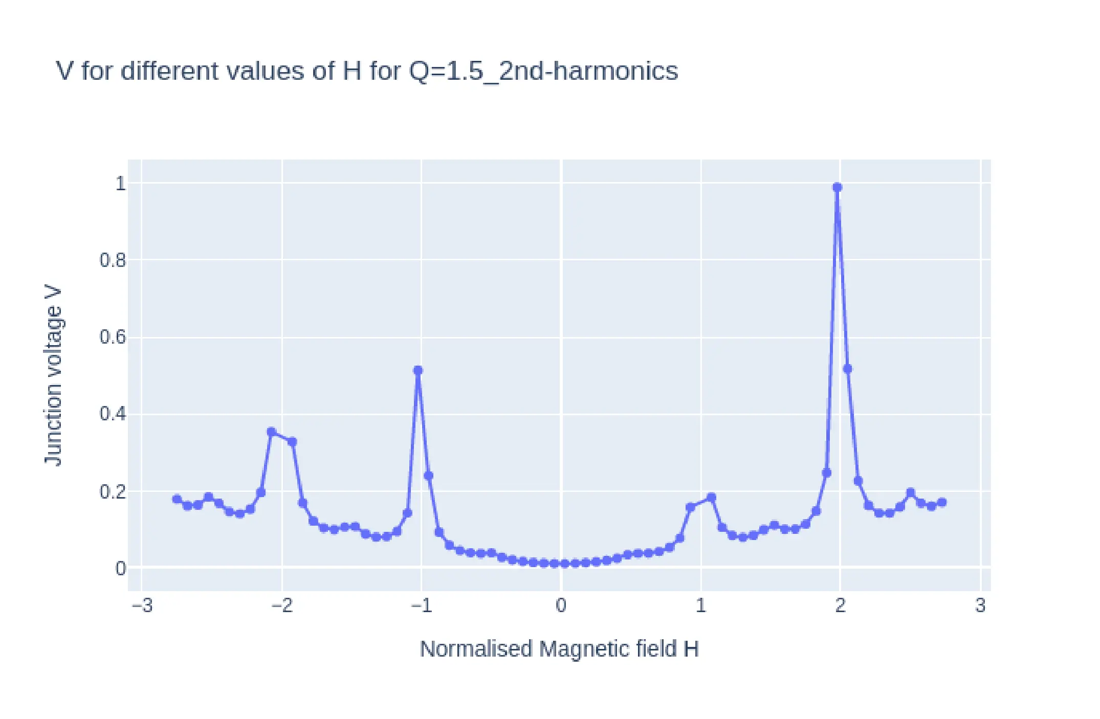
In Fig10, we see the plots of \(I_{c}H\) (top) and log plot of \(VH\) (bottom) from simulation with parameter Q=1.5 and second harmonics enabled. The \(I_{c}H\) and \(VH\) plots have similar shape at the key magnetic field points. ie the main lobe width and the side lobe widths are same. The characteristic second harmonic kinks appear at the same positions as well thus confirming the hypothesis that \(I_{c}H\)and \(VH\) (magnetoresistance) have similar characteristics for a Josephson junction. Fig 12 is the same plots of \(I_{c}H\)and \(VH\) for Q-1.5 but with only the first harmonics included. Here too the \(I_{c}H\)and \(VH\) (magnetoresistance) have similar characteristics further confirming the hypothesis.

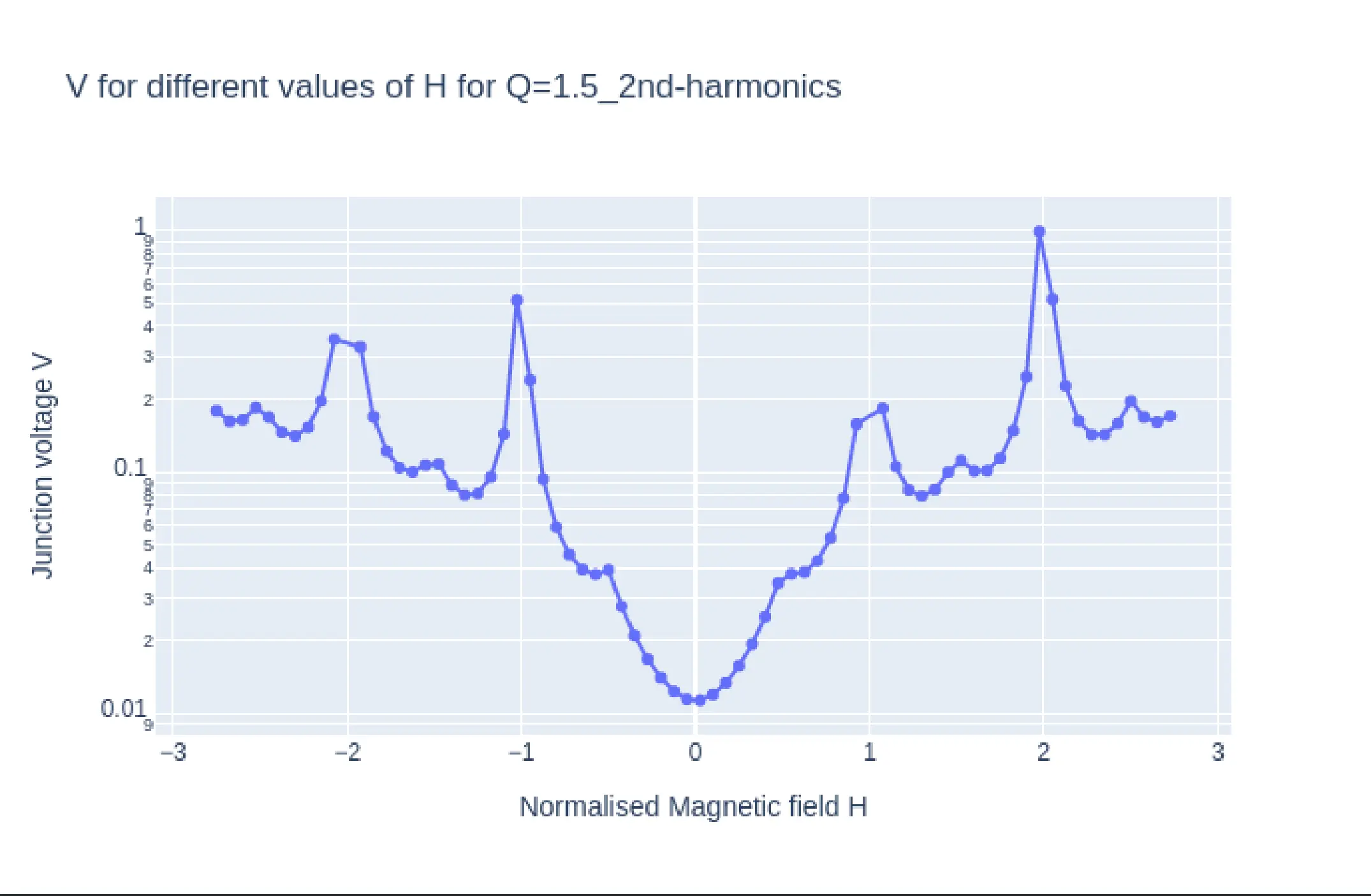
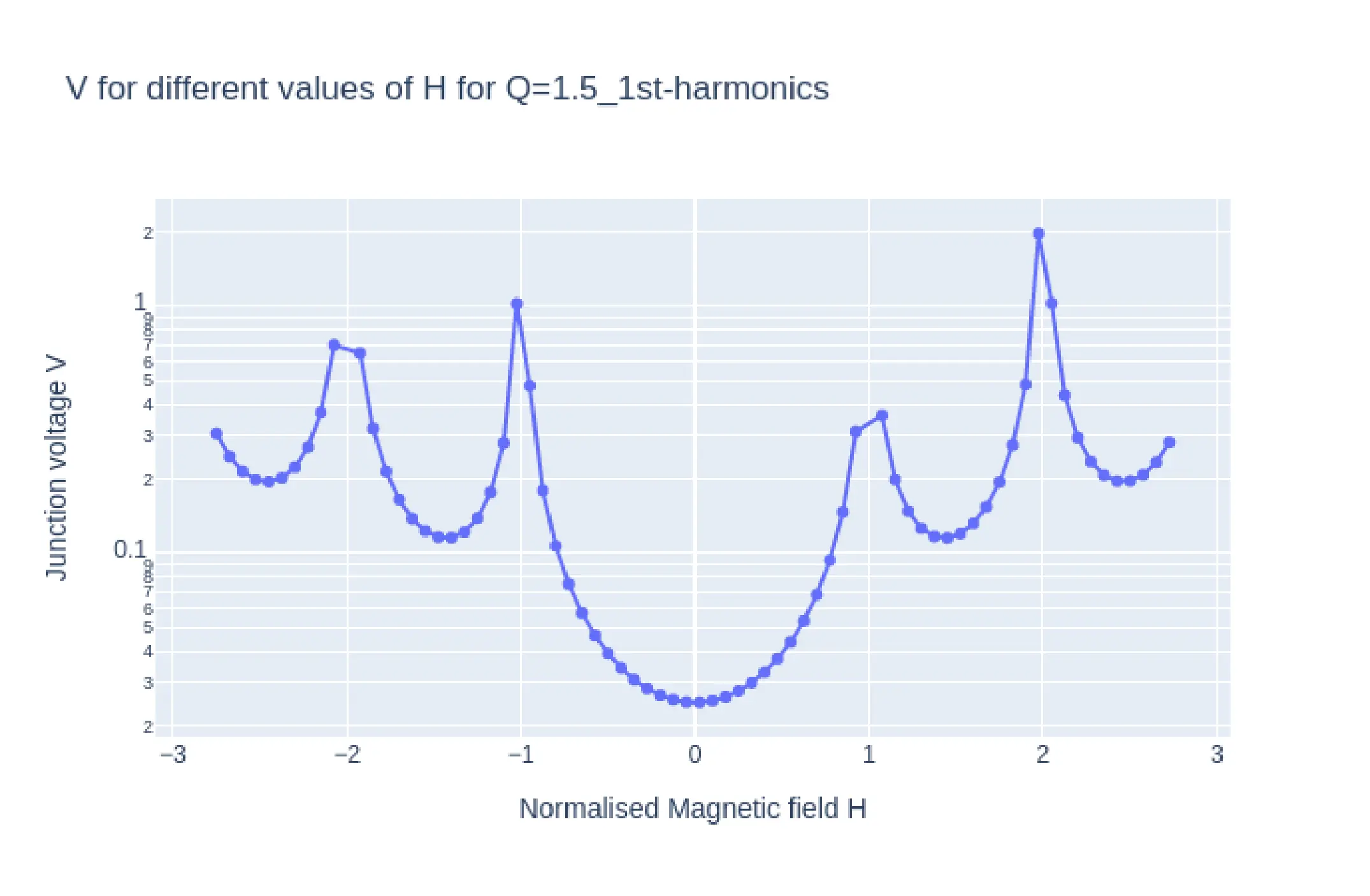
One must notice that the \(VH\) plots in bot the above figures have y axis in log scale. The reason for this is that for the selected Q=1.5 the junction resistance turns out to be extreamly large at 120\(\Omega\), the typical resistnace of a junction lies in the milli ohm range, thus the reported Voltages for the same current would be magnitudes higher, thus a log plot is taken inorder to correct this.

Experimental Measurements¶

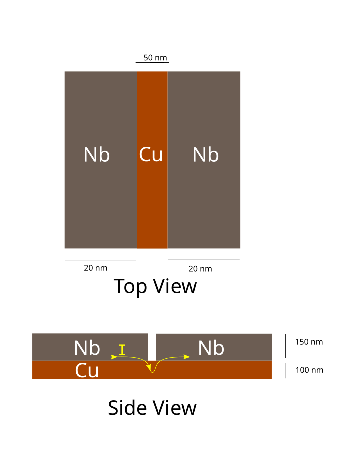
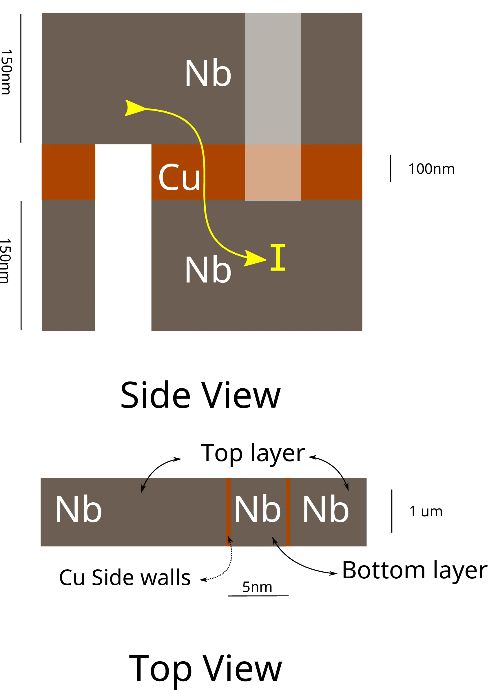
There are two geometries in which the Josephson junction are fabricated using FIB, one is the vertical Junction (Fig 15), and the other is the planar Junction (Fig 14); both names describe the path the current takes through the trilayers. In the planar Junction, the current is in plane with the trilayers and in the case of the vertical junctions the current flows vertically through the trilayers.

All the superconducting devices were first cooled to sub 2K, and then a 4 probe resistance vs temperature measurement was carried out with 1 - 10 \(\mu\)A by ramping the temperature slowly to 10K, in order to see the phase transitions. One such R-T graph is shown in Fig 16.

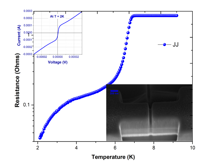
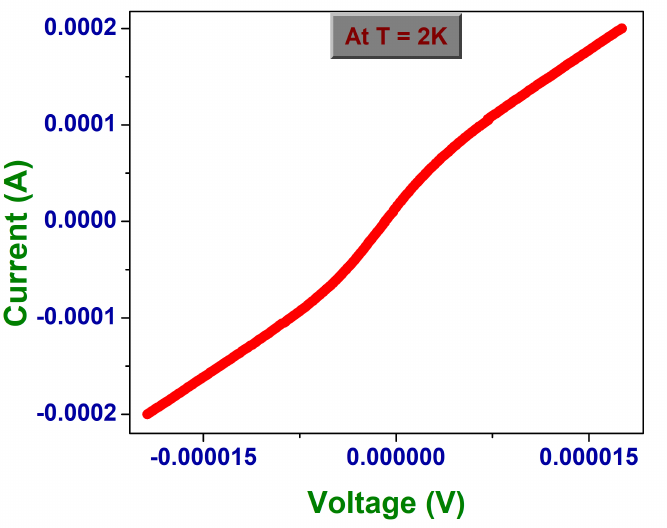
The first transition indicates the superconducting transition of the Niobium layer, and the second transition explains the proximitisation of the weak link. The resistance \(R_{n}\) at 9K (above \(T_{c}\)) and \(R_{L}\)at 2K are noted and the sample is cooled back to sub 2K. \(R_{n}\)is the normal resistance and indicates that the device is out of the superconducting regime. Once the devices cool down to 2K the current-voltage characteristics of the device is measured by sweeping current from -\(I_{n}\) to +\(I_{n}\), where \(I_{n}\) is the current for which the device yields the resistance \(R_{n}\) at 2K, ie. the device switches to the normal regime. The I-V curves have the typical JJ behavior and is plotted in Fig 17.

\(I_{c}\) of the device and the electrodes were extracted using the python scripts mentioned in section [subsec:Automation-of-].

In Fig 17 the IV curve of a Nb/Cu Josephson Junction is shown. Once the device \(I_{c}\) is found, the device is cooled to 2K and then supplied with \(I_{c}\) current, and the junction voltage is measured while ramping the magnetic field from +250 Oe to -250 Oe ( positive cycle ) and then from -250Oe to 250Oe ( negative cycle ) at 2K. This gives us magnetoresistance as a function of the applied magnetic field. The magnetoresistance as a function of applied magnetic field is expected to have a diffraction pattern for JJ. This was explained in the theoretical sections above.

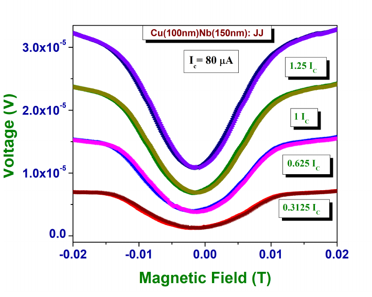
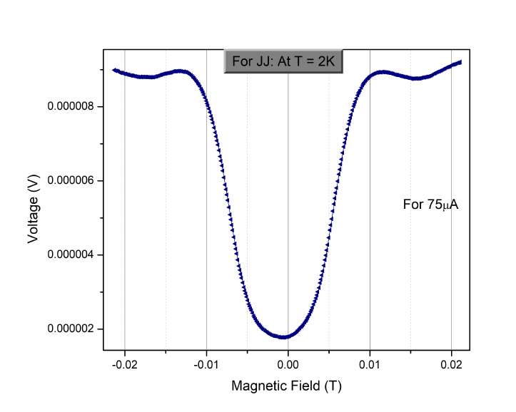
In Fig 19 , we examine the magnetoresistance of the patterned Nb/Cu Josephson junction device in low magnetic fields (|H| < 300 Oe) and at its \(I_{c}\). We find that the main lobe of the positive and the negative cycle overlap completely and there is no shift of the main lobe from origin as one would expect for a normal S-N-S junction. Fig 19 is a plot of Junction voltage as a function of magnetic field for another patterned Nb/Cu Josephson junction device in low magnetic fields for different values of junction currents. One can observe that higher currents increase the height of the lobes however the ratio of the first (main) lobe to the second lobe remains constant. This pattern was also confirmed with the simulation results.

Comparing simulation with experimental data¶

In Fig 19. Magnetoresistance of the patterned Nb/Cu Josephson junction device (which exhibits first harmonics only) in low magnetic fields for different values of junction currents is plotted. This plot is similar to the \(VH\) plot obtained from the simulation for Q=1.5 with only first harmonics enabled (Fig 12 (bottom) ). This further confirms the equivalence between \(VH\) plot obtained experimentally and \(VH\) plot obtained from simulations, Thus establishing that the \(VH\) plot obtained experimentally confirms the typical characteristic of the Josephson junction.

Processing experimental data¶

Automation of \(I_{c}\) extraction¶

Once the IV simulation is done, in order to aggregate data for \(I_{c}\)as a function of applied magnetic field \(H\) (\(I_{c}H)\) and Junction voltage at as a function of applied magnetic field \(H\) (\(VH\)), One must first set the process for identifying \(I_{c}\). In case of simulations, since the data is quite smooth, we could choose a junction voltage which corresponds to Ic for one run and find the current value for that particular voltage on other runs. This is essentially a horizontal slice of the IV curve in Fig 4. For experimental data, there is another way to define the \(I_{c}\)of a given PPMS data.

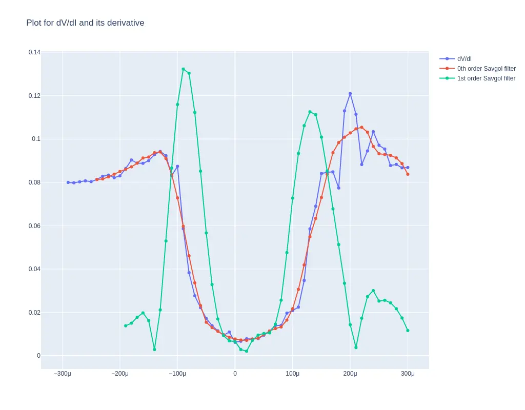
\(I_{c}\) of the junction were extracted from this data by running through a python script that takes in the I-V data, calculates dV/dI, and applies a Savitzky–Golay filter of first-order to obtain \(d^{2}I/d^{2}V\) and find the current (\(I_{c}\)) for which \(d^{2}I/d^{2}V\) in both the positive and negative side and averages them. For normal Josephson junction the position of peak of \(dI/dV\) is a good marker of the \(I_{c}\), however in cases where the junction resistance is high, \(dI/dV\) might not be clear enough to mitigate this peaks of \(d^{2}I/d^{2}V\) is a better marker of \(I_{c}\) A sample graph of \(dI/dV\) and \(d^{2}I/d^{2}V\) for a I vs V curve measured on a Josephson junction is shown in Fig 20.

The code for the python script is available here and a web app based on the same is hosted at jj-ic-finder.streamlit.app

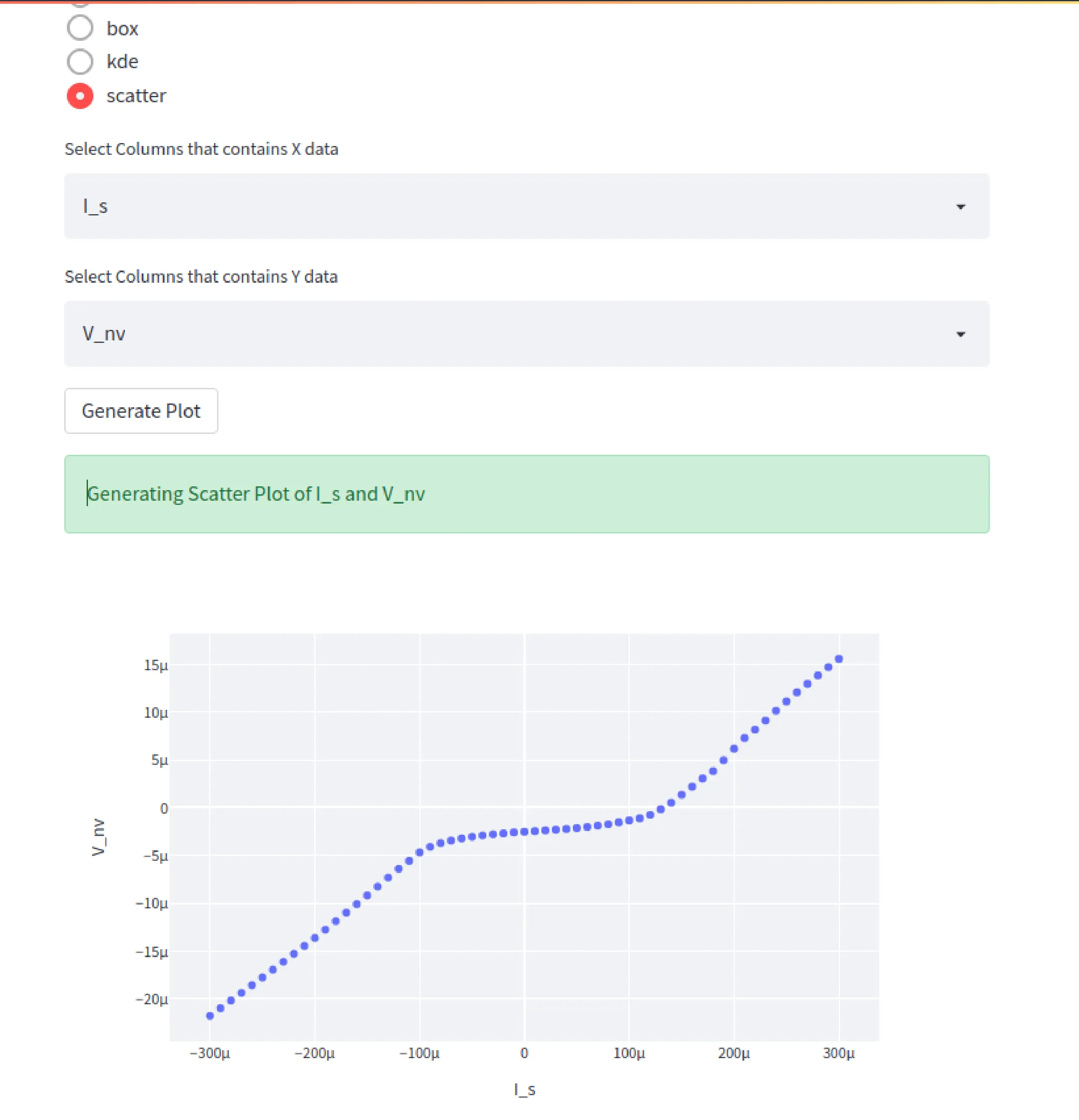
The web app also provides quick access to multiple data visualizations like area plot,bar plot,line plot, hist plot, scatter plot etc. A screenshot of the web-app in use for visualizing the IV of an experimental data of JJ is shown in Fig21.

Inferring \(I_{c}\) behavior via repetitive IV measurement¶

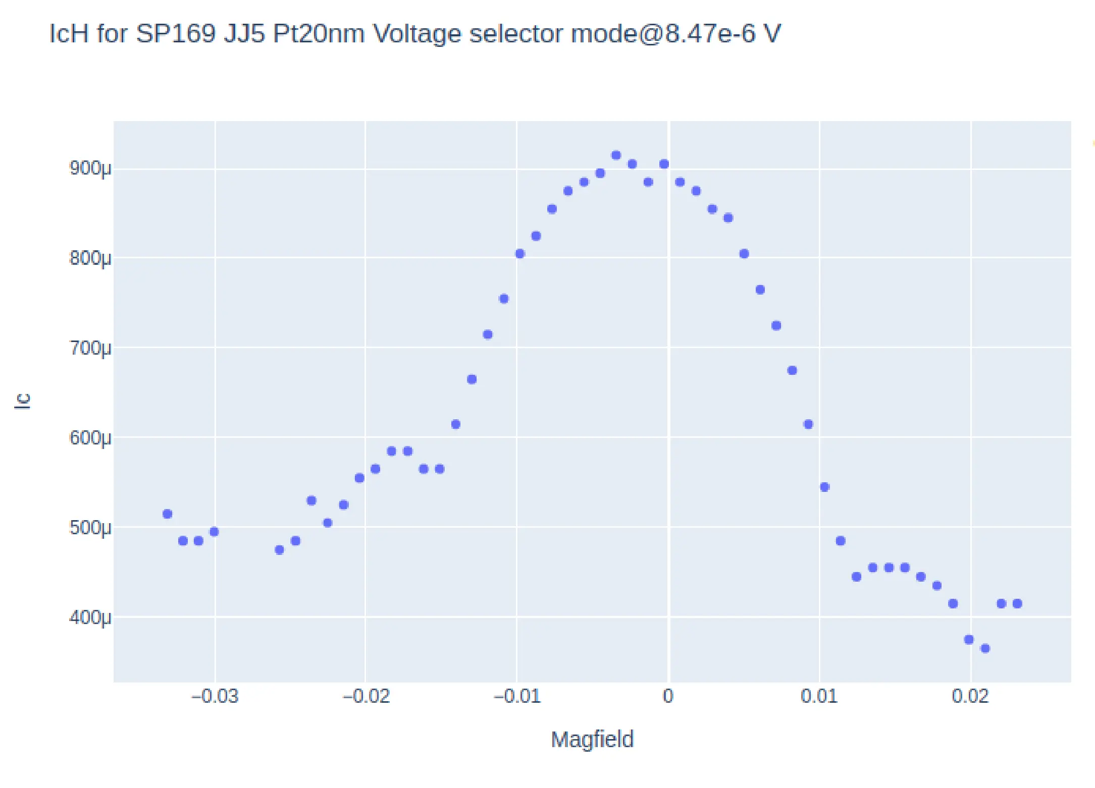
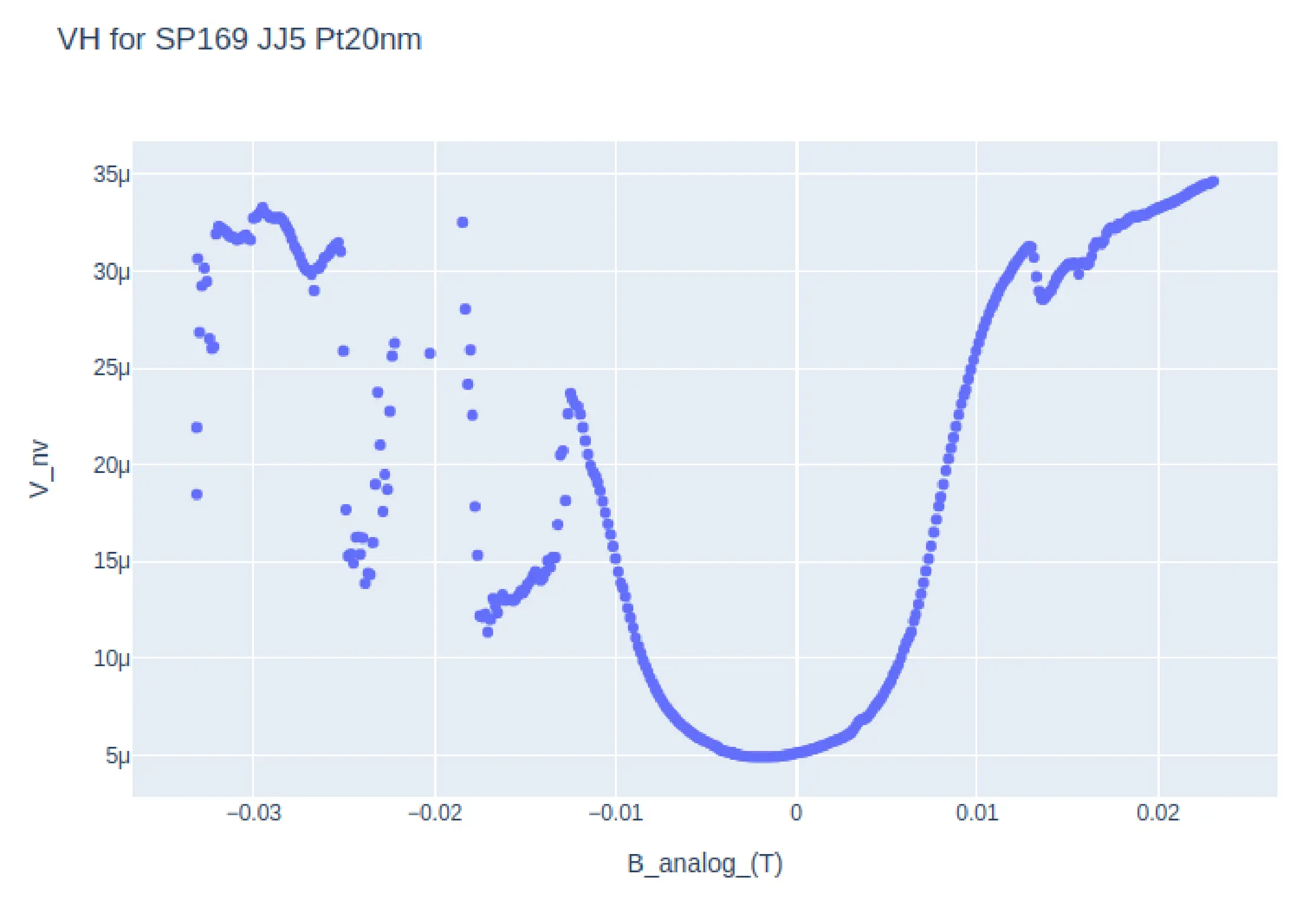
The characteristic signature of a Josephson junction, apart from its current voltage relation (IV) is the Critical current \(I_{c}\)dependence on the applied magnetic field H ( \(I_{C}\)vs H or \(I_{C}H\)).

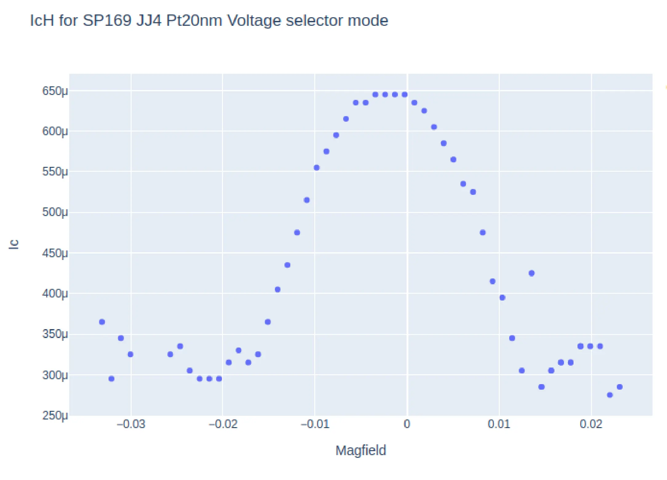
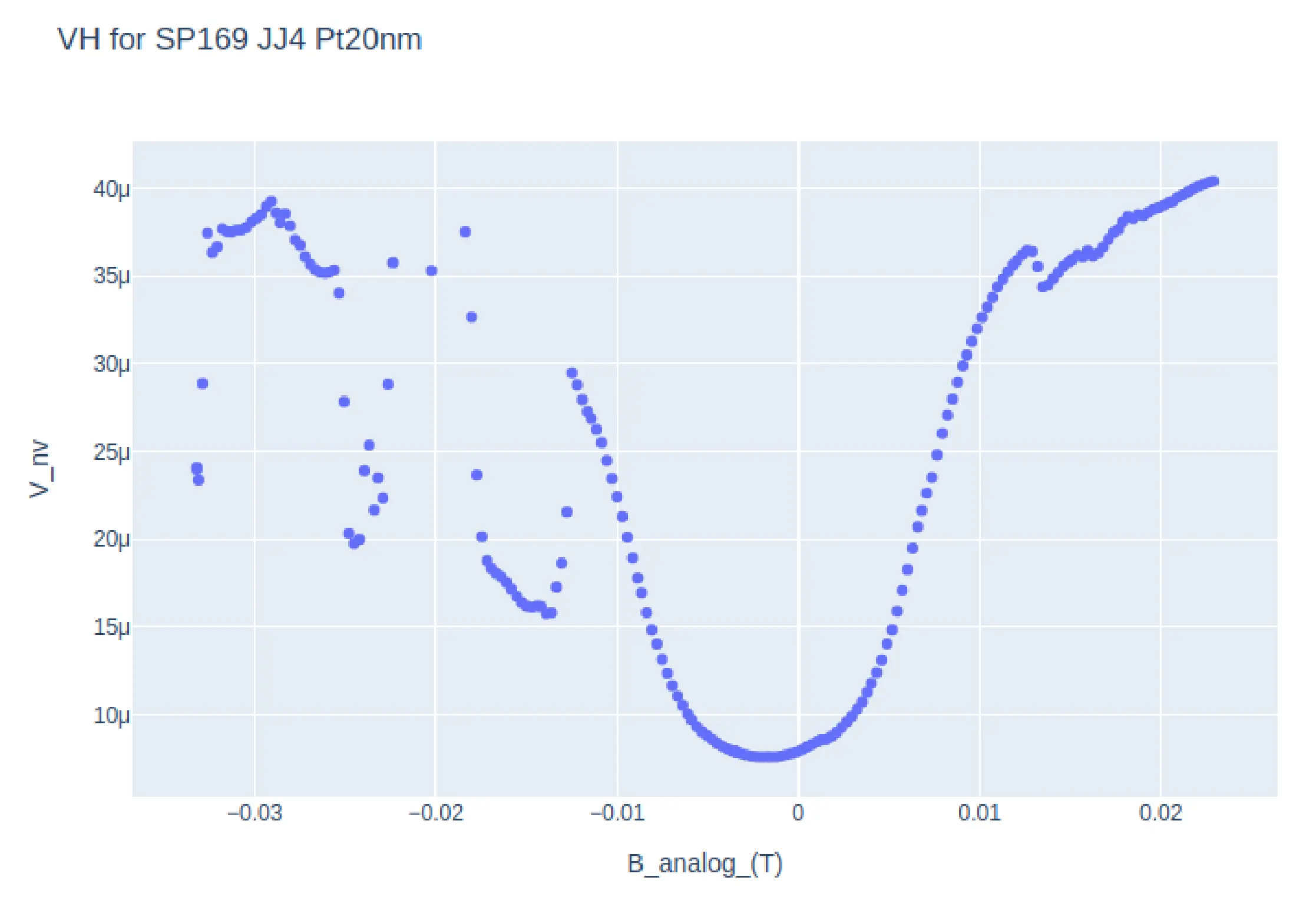
The PPMS in the lab has builtin recipes only for DC measurement and as such DC measurements like IV are relatively slower (1 IV scan in 10-15 minutes on good resolution). Thus getting data for \(I_{c}H\) would require multiple IVs to be measured at a sweep of magnetic field H. This would take almost a day per device on a decent resolution and thus cant be done frequently. The more easier measurement would be to set and constant current (say the \(Ic\) at zero magnetic field) then measure the Voltage as a function of changing magnetic field ( V vs H or VH ) however, there is little literature regarding the VH relation (or magneto resistance ) of a Josephson junction. In order to verify the correlation between the \(I_{C}H\) and \(VH\) signatures of a Josephson junction, apart from the simulation methods, multiple IV seeps of a Josephson Junction were setup at varying magnetic field were taken, and a python script mentioned in the previous sub section was used to identify the \(I_{C}\) for each \(H\). The plots of these \(I_{C}H\) and \(VH\) data is shown in Fig . The VH data for these junctions have some parts which are offset due to random phase jumps. On comparison, one can make out the Fraunhofer like pattern in both plots at the same magnetic field points, the main lobe width and the secondary lobe width are identical.

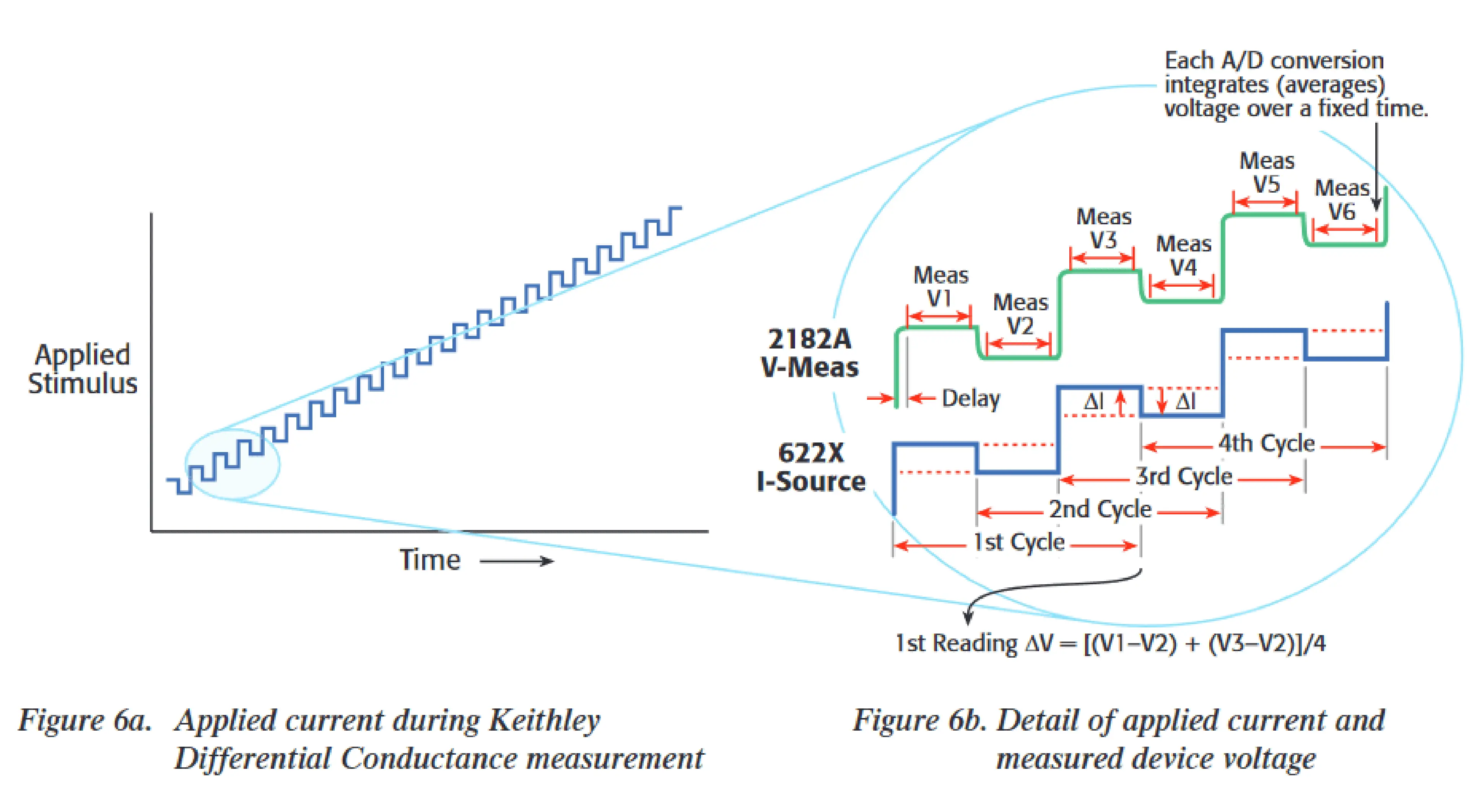
Apart from this measurement, an attempt was made to setup Keithley 6221 - AC current source and Keithley 2182a - Nanovoltmeter in differential conductance mode.

This method involves sweeping a linear staircase profile with an alternating current. The differential current, dI, is the amplitude of the alternating portion of the current as shown in Fig 26. Throughout the test, the differential current remains constant. A Trigger Link cable synchronises the current source with the nanovoltmeter. The nanovoltmeter calculates the delta voltage between consecutive steps after measuring the voltage at each current step. To determine the differential voltage, dV, each delta voltage is averaged with the previous delta voltage. dI/dV may now be used to calculate the differential conductance, dG. (“Achieving Accurate and Reliable Resistance Measurements in Low Power and Low Voltage Applications Tektronix” n.d.)

The Labview program provided by the instrument manufacturer required the connection to the 6221 via a GPIB interface, however the 6221 was connected to a system with no GPIB port. In order to over come this, communication was setup serially via the Ethernet ports and python serial communication library. A graphical user interface (GUI) was built built to control the communication and perform the differential conductance as shown in Fig 27.

The data provided by the instrument is differential conductance, dG as a function of applied current. The experiment needed dG as a function of junction voltage and the data acquired by the device was quite unreliable and noisy, thus this method was not used further. A better way to do differential conductance would be to use a lock-in amplifier.

Conclusion¶

The main goal of the thesis was to establish equivalence between the \(I_{c}H\)and \(VH\) (magnetoresistance) characteristics of a Josephson junction ( with and without the second harmonics), then further establish the experimental \(VH\) plot and the simulated \(VH\) plot.

For the first part, the simulation was setup by solving the ODE with input similar to the experimental input of, sweeping the current while equilibrating the system at each step and then repeating this over multiple magnetic field, then further analysing this data to obtain \(I_{c}H\)and \(VH\) plots. For the second part, experimental data was gathered similar to the simulation steps (calculating IV data for multiple magnetic field ) and then analysed to to obtain \(I_{c}H\)and \(VH\) plots, the results obtained from this was matched with the simulation results.

In both of the above method, the equivalence between the \(I_{c}H\)and \(VH\) (magnetoresistance) characteristics of a Josephson junction was confirmed and was also matched with the experimental results. One could carry out the study further by:

• Carrying out a simulation analysis with respect to \(\beta_{c}\)and compare it with the results obtained through Q

• Simulation of other exotic CPR such as sin(\(\phi/2\))

• The simulation currently takes about 2hrs for sweeping magnetic fields linearly spaced between \(-2\frac{\phi}{\phi_{0}}\) and \(2\frac{\phi}{\phi_{0}}\) . An improvement in the simulation/integration time by using numba decorators for numpy-python modules could be made, for instance Scipy’s odeint integration will be slow if the right-hand side of an ODE integration is slow. The numba package, which translates python code into machine code using LLVM - which means it’s very fast, it can speed up the right-hand side. Even a very simple ODE can be sped up by several factors.

• A study could be done on finding the Q value of the experimental junction, by fitting the IV with Q as a parameter

• The differential conductance measurement could be setup using a lockin amplifier.

References¶

“Achieving Accurate and Reliable Resistance Measurements in Low Power and Low Voltage Applications Tektronix.” n.d. Accessed May 9, 2022. https://www.tek.com/en/documents/whitepaper/achieving-accurate-and-reliable-resistance-measurements-low-power-and-low-voltag.

Assouline, Alexandre, Cheryl Feuillet-Palma, Nicolas Bergeal, Tianzhen Zhang, Alireza Mottaghizadeh, Alexandre Zimmers, Emmanuel Lhuillier, et al. 2019. “Spin-Orbit Induced Phase-Shift in Bi2Se3 Josephson Junctions.” Nature Communications 2019 10:1 10 (January): 1–8. https://doi.org/10.1038/s41467-018-08022-y.

Bardeen, J., L. N. Cooper, and J. R. Schrieffer. 1957. “Theory of Superconductivity.” Phys. Rev. 108 (December): 1175–1204. https://doi.org/10.1103/PhysRev.108.1175.

DanielSank. n.d. “What Does the \(I\)-\(V\) Curve in Josephson Junction Mean?” Physics Stack Exchange. https://physics.stackexchange.com/q/197150.

Drozdov, A. P., M. I. Eremets, I. A. Troyan, V. Ksenofontov, and S. I. Shylin. 2015. “Conventional Superconductivity at 203 Kelvin at High Pressures in the Sulfur Hydride System.” Nature 525 (7567): 73–76. https://doi.org/10.1038/nature14964.

Frolov, S. M., D. J. Van Harlingen, V. A. Oboznov, V. V. Bolginov, and V. V. Ryazanov. 2004. “Measurement of the Current-Phase Relation of Superconductor/Ferromagnet/Superconductor Pi Josephson Junctions.” Phys. Rev. B 70 (October): 144505. https://doi.org/10.1103/PhysRevB.70.144505.

Josephson, B. D. 1962. “Possible New Effects in Superconductive Tunnelling.” Physics Letters 1 (7): 251–53. https://doi.org/10.1016/0031-9163(62)91369-0.

Khan, Jamal Akhtar, and M. Shahabuddin. 2009. “Simulation Study of Effect of Magnetic Field over i-v Characteristic of Intrinsic Stacked Josephson Junctions.” International Journal of Nanomanufacturing 4 (1/2/3/4): 342. https://doi.org/10.1504/ijnm.2009.028142.

Klenov, N, V Kornev, A Vedyayev, N Ryzhanova, N Pugach, and T Rumyantseva. 2008. “Examination of Logic Operations with Silent Phase Qubit.” Journal of Physics: Conference Series 97 (February): 012037. https://doi.org/10.1088/1742-6596/97/1/012037.

Lee, Gil-Ho, and Hu-Jong Lee. 2018. “Proximity Coupling in Superconductor-Graphene Heterostructures.” Reports on Progress in Physics 81 (5): 056502. https://doi.org/10.1088/1361-6633/aaafe1.

Ngo, Duc-The. 2021. “Lorentz TEM Characterisation of Magnetic and Physical Structure of Nanostructure Magnetic Thin Films,” December.

Pal, Avradeep, Z. H. Barber, J. W. A. Robinson, and M. G. Blamire. 2014. “Pure Second Harmonic Current-Phase Relation in Spin-Filter Josephson Junctions.” Nature Communications 5 (1). https://doi.org/10.1038/ncomms4340.

Rowell, J. M. 1963. “Magnetic Field Dependence of the Josephson Tunnel Current.” Phys. Rev. Lett. 11 (September): 200–202. https://doi.org/10.1103/PhysRevLett.11.200.

Schmidt, F. E. 2017. “RCSJ.” https://github.com/feschmidt/rcsj.

Schrieffer, J. R., and M. Tinkham. 1999. “Superconductivity.” Rev. Mod. Phys. 71 (March): S313–17. https://doi.org/10.1103/RevModPhys.71.S313.

Sellier, Hermann, Claire Baraduc, François Lefloch, and Roberto Calemczuk. 2004. “Half-Integer Shapiro Steps at the 0-Pi Crossover of a Ferromagnetic Josephson Junction.” Phys. Rev. Lett. 92 (25 Pt 1): 257005.

Stoutimore, M J A, A N Rossolenko, V V Bolginov, V A Oboznov, A Y Rusanov, D S Baranov, N Pugach, S M Frolov, V V Ryazanov, and D J Van Harlingen. 2018. “Second-Harmonic Current-Phase Relation in Josephson Junctions with Ferromagnetic Barriers.”

Strambini, Elia, Andrea Iorio, Ofelia Durante, Roberta Citro, Cristina Sanz-Fernández, Claudio Guarcello, Ilya V Tokatly, et al. n.d. “A Josephson Phase Battery.” Nature Nanotechnology. https://doi.org/10.1038/s41565-020-0712-7.

Tanaka, Yukio, and Satoshi Kashiwaya. 1997. “Theory of Josephson Effects in Anisotropic Superconductors.” Phys. Rev. B 56 (July): 892–912. https://doi.org/10.1103/PhysRevB.56.892.

Wang, Lujun. 2015. “Fabrication Stability of Josephson Junctions for Superconducting Qubits.” In.

Yamashita, T., K. Tanikawa, S. Takahashi, and S. Maekawa. 2005. “Superconducting \(\ensuremath{\pi}\) Qubit with a Ferromagnetic Josephson Junction.” Phys. Rev. Lett. 95 (August): 097001. https://doi.org/10.1103/PhysRevLett.95.097001.

Acknowledgments¶

I wish to thank my project supervisors, Dr. Kartikeswar Senapati and Dr. Ramesha C K for their immense support and help with the understanding of this project. I would like to express my deepest appreciation to Mr. Tapas Ranjan Senapati and Ms. Laxmipriya Nanda for all their help from mentoring on the fabrication techniques to usage of measurement systems and all the fruitful discussions. I wish to thank all the lab members of Superconductivity lab, NISER for all the brainstorming sessions which helped me greatly. Special thanks to Ms. Soheli Mukherjee who always supported me with all my endeavors. I would also like to extend my deepest gratitude to Dr. Dhavala Suri who always showered me with helpful advice. Lastly, I am thankful to all my friends and family members for extending their love and support.

Abbreviations¶

• AC :- Alternating current

• RF :- Radio frequency

• JJ :- Josephson Junction

• SQUID :- Superconducting QUantum Interference Device

• EDX :- Energy Dispersive X-ray spectroscopy

• SEM :- Scanning Electron Microscope

• FIB :- Focused Ion Beam

• PPMS :- Physical Properties Measurement System

• Fig :- Figure

• eV :- Electron Volt

• KeV :- Kilo Electron Volt

• MeV :- Mega/Million Electron Volt

• et al :- And others (Latin)

• i.e. :- That is

• etc :- Et cetera (Latin for ’and others of same kind’)

• T :- Tesla

• SiO2:- Silicon dioxide

• R-T :- Resistance Versus Temperature

• I-V :- Current Versus Voltage

• I-H :- Current Versus Magnetic field

• V-H :- Voltage Versus Magnetic field

• Si :- Silicon

• K :- kelvin

• mm :- millimeter

• mbar :- millibar

• IPA :- Isopropyl alcohol

• RPM :- Revolutions Per Minute

• C :- Celsius

• Ar :- Argon

• e.g. :- Example given

• TSP :- Titanium Sublimation Pump

• RGA :- Residual Gas Analyzers

• Cu :- Copper

• BCS :- Bardeen–Cooper–Schrieffer

• Nb :- Niobium

• DC :- Direct current

• AC :- Alternating current

• \(\mu\)A :- Micro Ampere

• \(\Omega\):- Ohm

• nm :- Nano meter